Neural Machine Translation Inside Out
 This is a blog version of my talk at the ACL 2021 workshop
Representation
Learning for NLP (and updated version
of that at NAACL 2021 workshop
Deep Learning Inside Out (DeeLIO)).
This is a blog version of my talk at the ACL 2021 workshop
Representation
Learning for NLP (and updated version
of that at NAACL 2021 workshop
Deep Learning Inside Out (DeeLIO)).
In the last decade, machine translation shifted from the traditional statistical approaches with distinct components and hand-crafted features to the end-to-end neural ones. We try to understand how NMT works and show that:
- NMT model components can learn to extract features which in SMT were modelled explicitly;
- for NMT, we can also look at how it balances the two different types of context: the source and the prefix;
- NMT training consists of the stages where it focuses on competences mirroring three core SMT components.
 July 2021
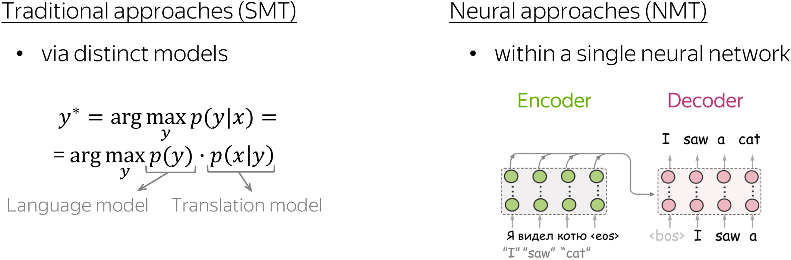
Machine Translation Task: Traditional vs Neural Mindsets
In the last decade, machine translation came all the way from traditional statistical approaches to end-to-end neural ones. And this transition is rather remarkable: it changed the way we think about the machine translation task, its components, and, in a way, what it means to translate.
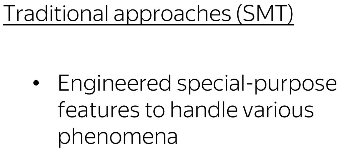
Traditional approaches split the translation task into several components: here humans decide which competences a model needs. In SMT, translation is split into target-side language modeling (which helps a model to generate fluent sentences in the target language) and a translation model (which is responsible for the connection to the source). The translation model, in turn, is split into lexical translation and alignment. Usually, there are also lots of hand-crafted features. Note that here the components and features are obtained separately and then combined in a model.
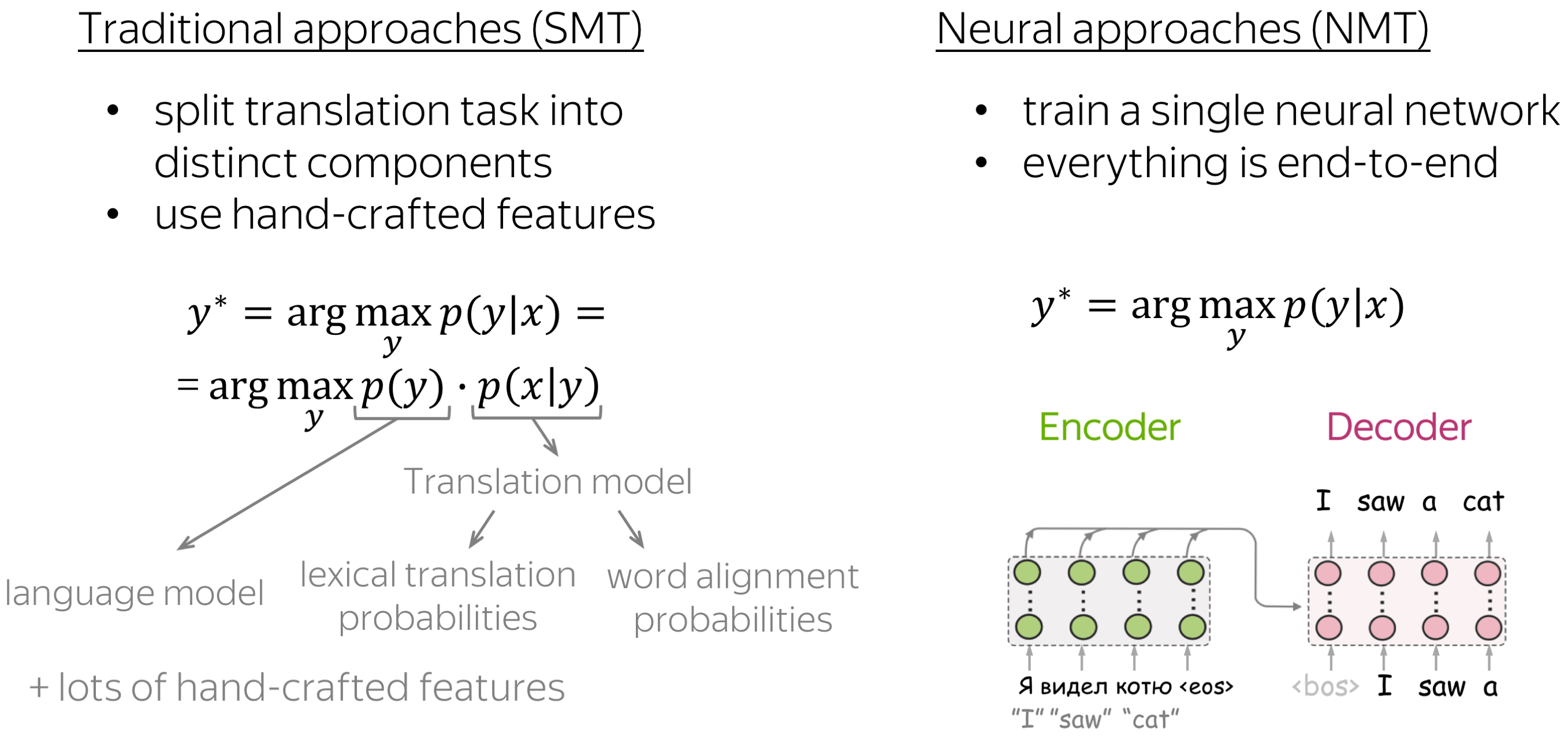
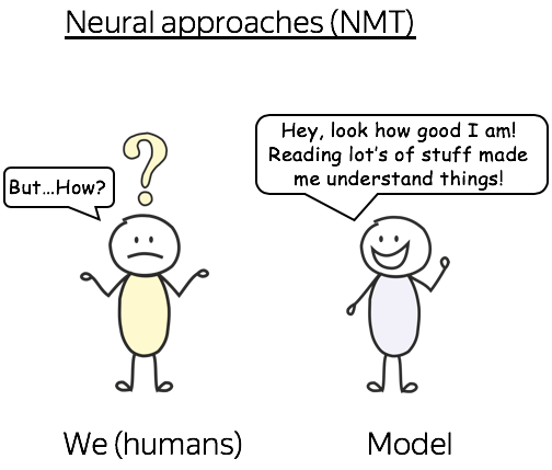
In neural approaches, everything is end-to-end: there is a single neural network that just reads lots of parallel data and somehow gets to learn the translation task directly, without splitting it into subtasks.
From Humans to Model, or From Model to Humans?
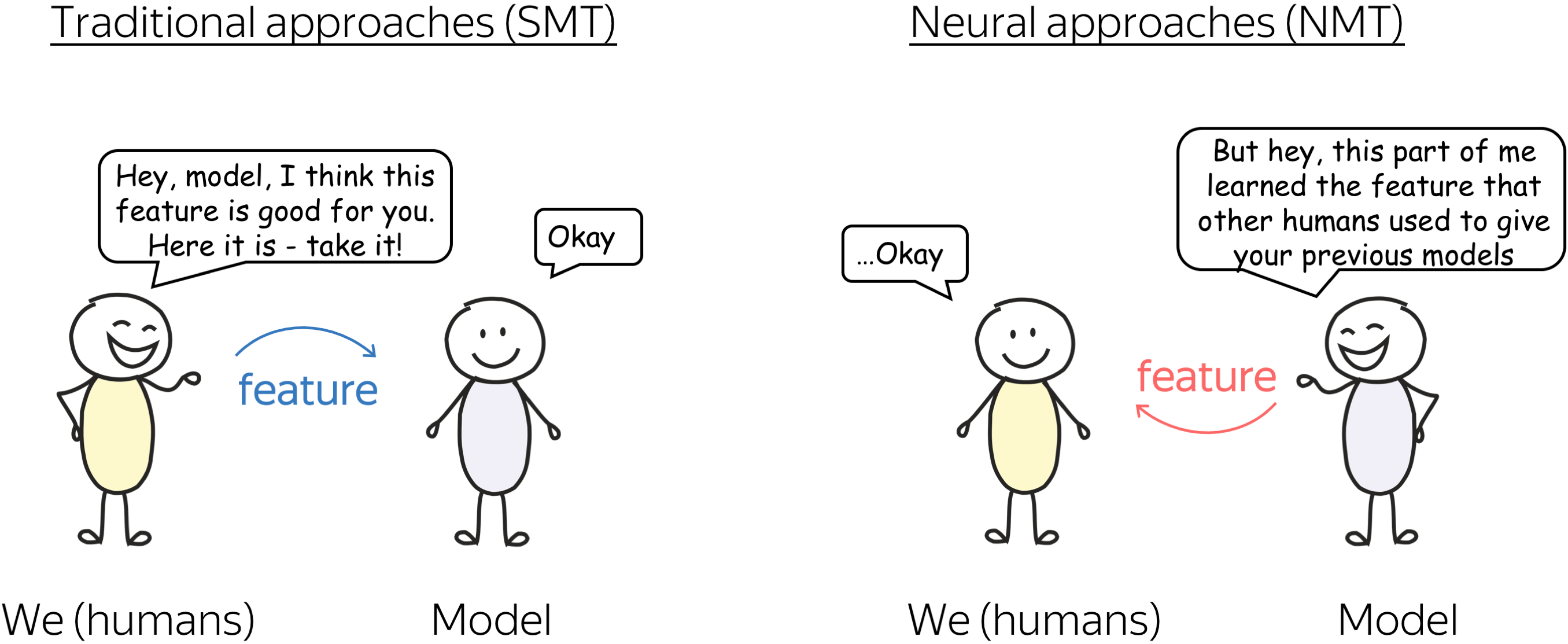
Let me give you an intuitive illustration of the differences between these two mindsets. In the two approaches, we have humans and a model. In SMT, humans tell the model: “Hey, model, take this and that and this other stuff - this is how you solve the task”. And the model replies “Okay” (well, what else can it do, right?)
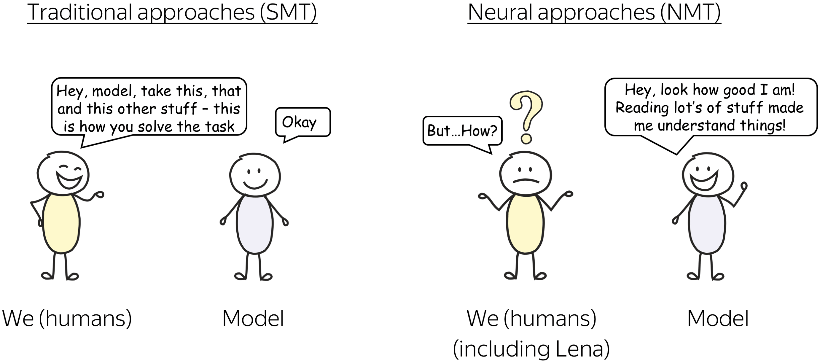
In NMT, the model tells us: “Hey, look how good I am! Reading lots of stuff made me understand things!”
And here we are: confused, surprised, and asking “How?”
The question of “How?” is the main question of this talk :) I look at it keeping in mind how things used to be done in SMT. From this perspective, there can be different questions:
- Can NMT model components take the roles mirroring SMT components and/or features?
- How does NMT balance being fluent (target-side LM) and adequate (translation model)?
- How does NMT acquire different competences during training, and how does this mirror the different models in traditional SMT?
Model Components and their Roles
Lena: This part will be high-level, just to illustrate the main idea. The two other questions we'll discuss in more detail.
The example is from:
Neural Machine Translation
by Jointly Learning to Align and Translate.
Here our question is:
Can NMT model components take the roles mirroring SMT components or features?
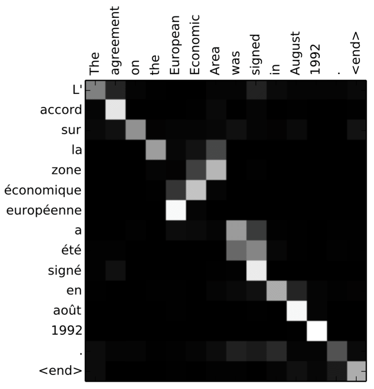
Of course they can - everybody knows that! Decoder-encoder attention is closely related to word alignment.
But don't worry: I have something more interesting for you:
Context-Aware NMT Learns Anaphora Resolution
Lena: This part is based on our ACL 2018 paper Context-Aware Neural Machine Translation Learns Anaphora Resolution.
What is Context-Aware NMT?
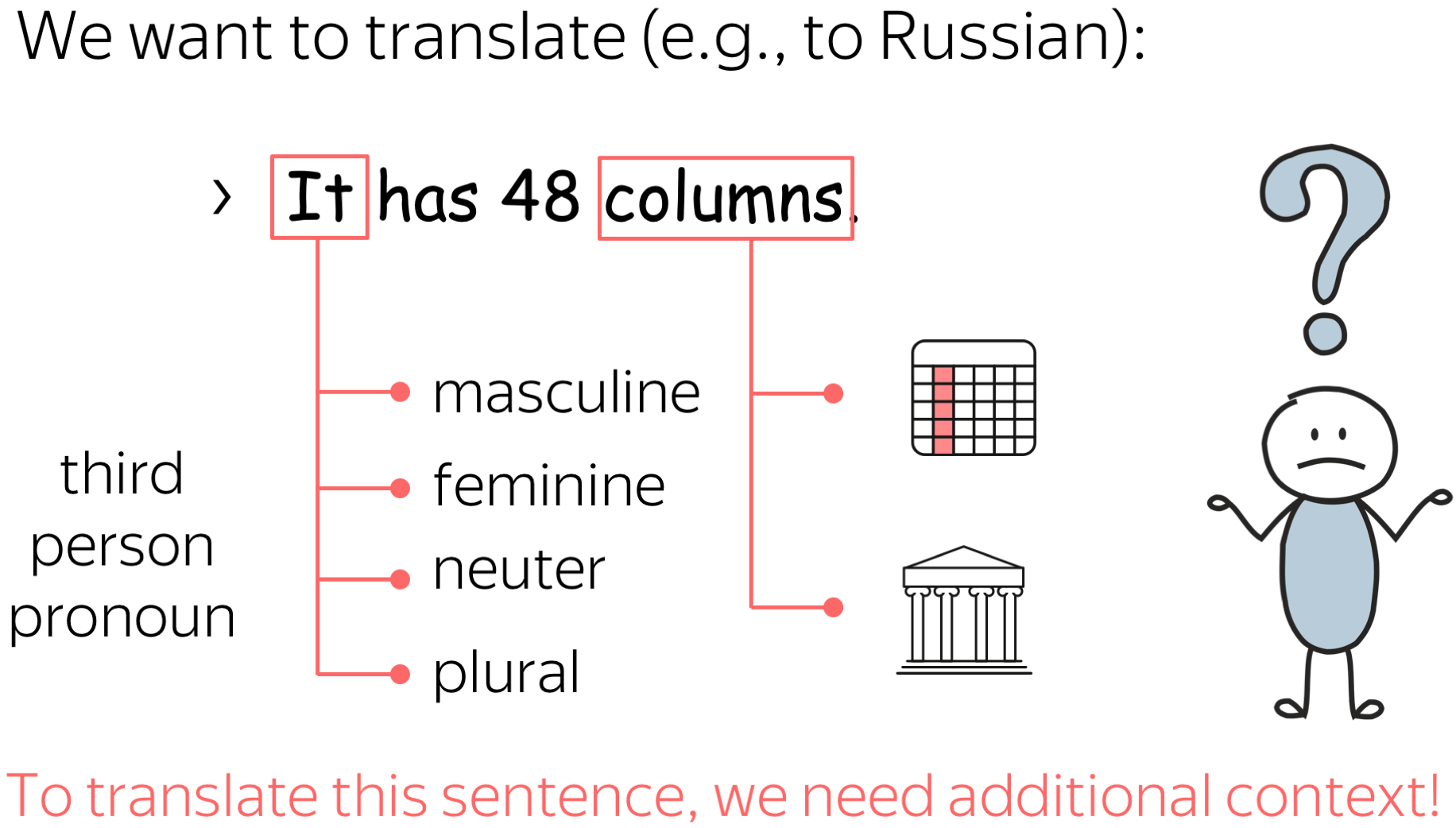
Standard NMT processes a single source sentence and generates the target sentence. But sometimes, the source sentence does not contain enough information to translate it. For example, here our source sentence contains the pronoun "it" which can have several correct translations into Russian (or any other language with gendered nouns) and to translate it we need to know what it means: for this, we need additional context. Also, the word "columns: is ambiguous and can have several correct translations.
Context-Aware NMT Model with Limited Interaction with Context
What we do, is we take one previous sentence, and plug it in. Specifically, we take the standard Transformer and in the final encoder layer, we add one attention layer to the context sentence.
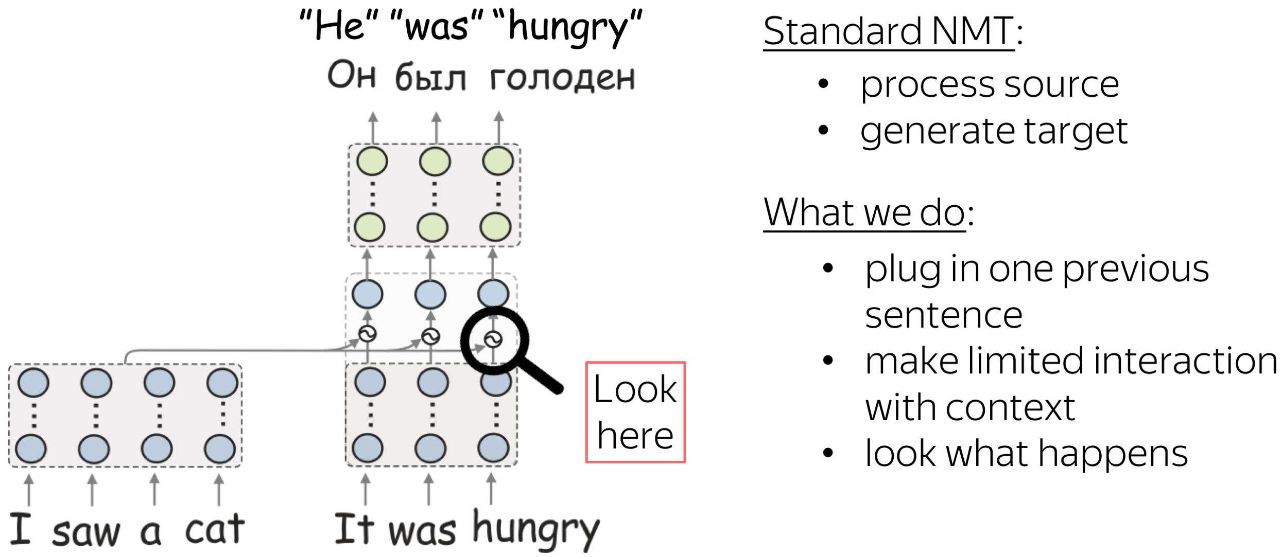
Note that we design very limited interaction with context to be able to look at what happens.
We got some improvements in quality, but this is not what we care about. We are interested in whether model components can learn something interesting. So let’s look at the attention to context. Since the model interacts with the context only through this attention layer, we can see what information the model takes from context.
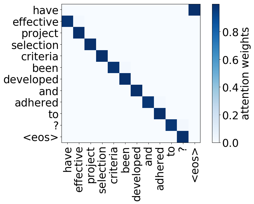
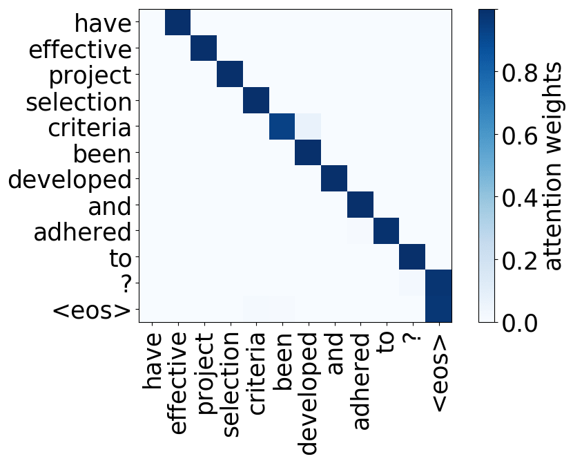
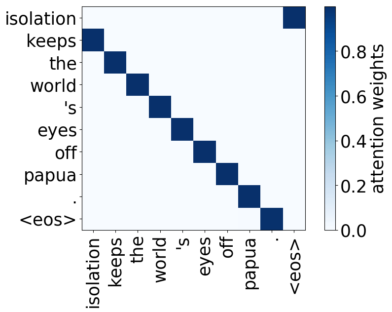
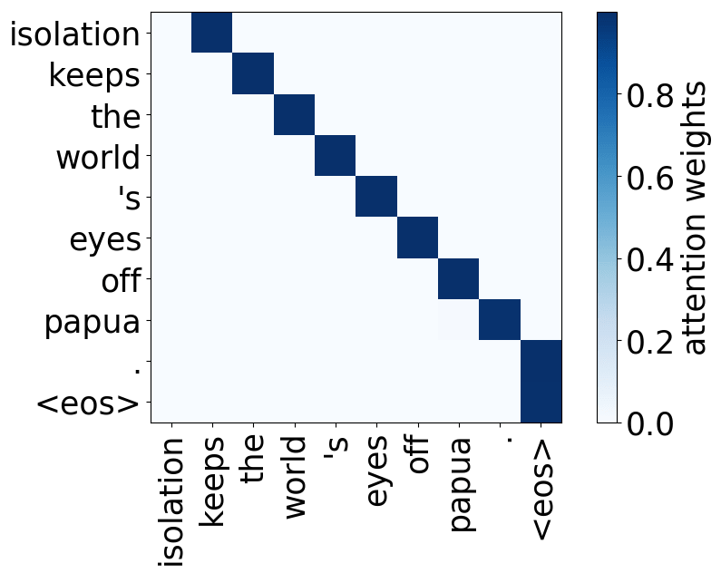
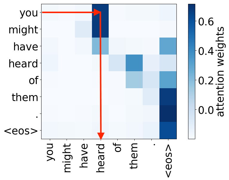
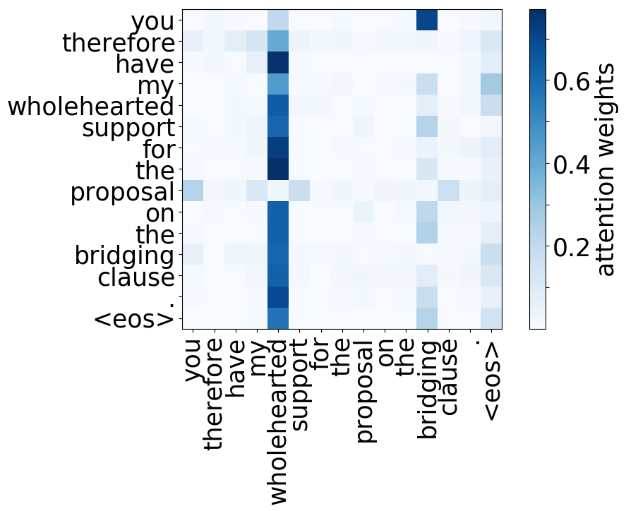
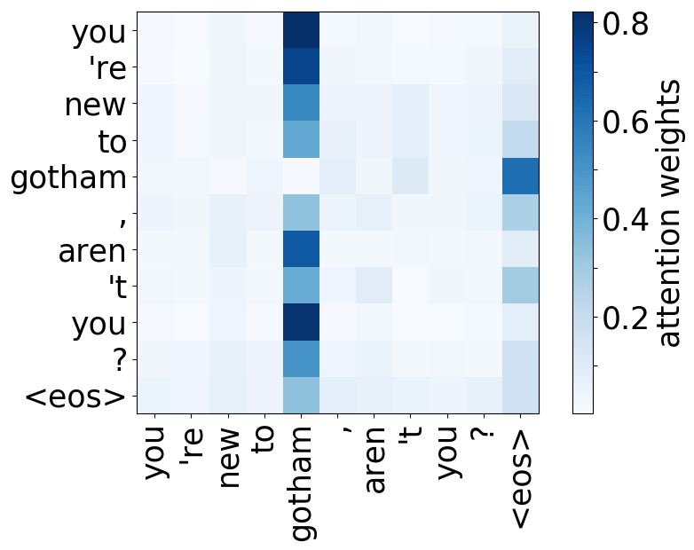
Attention Learned to Resolve Anaphora!
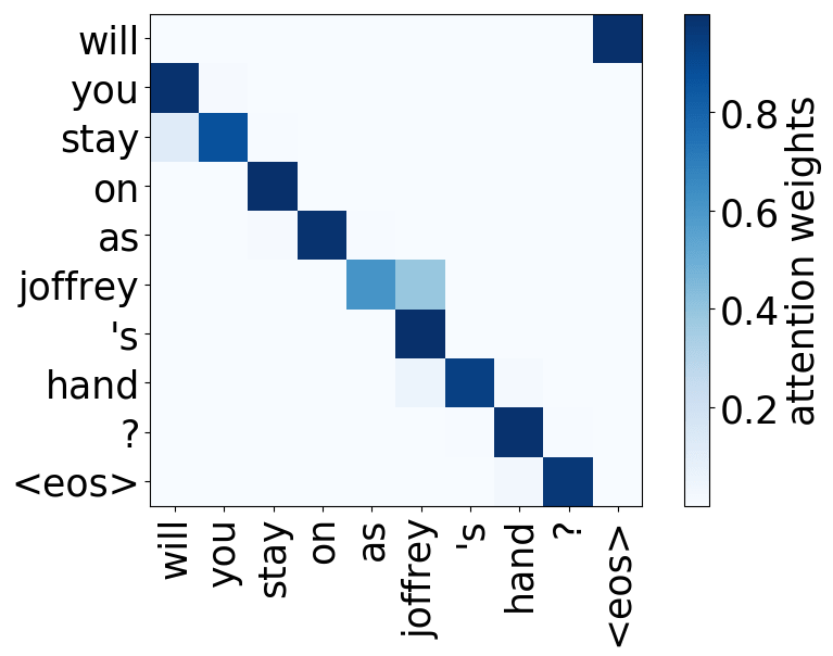
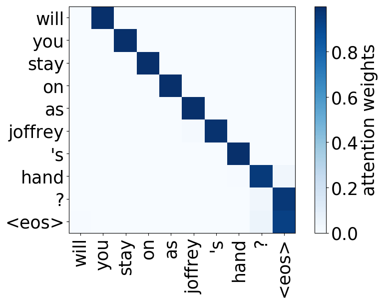
Let's look at the example of two consecutive sentences: the first is the context, the second is the source, the one we need to translate.
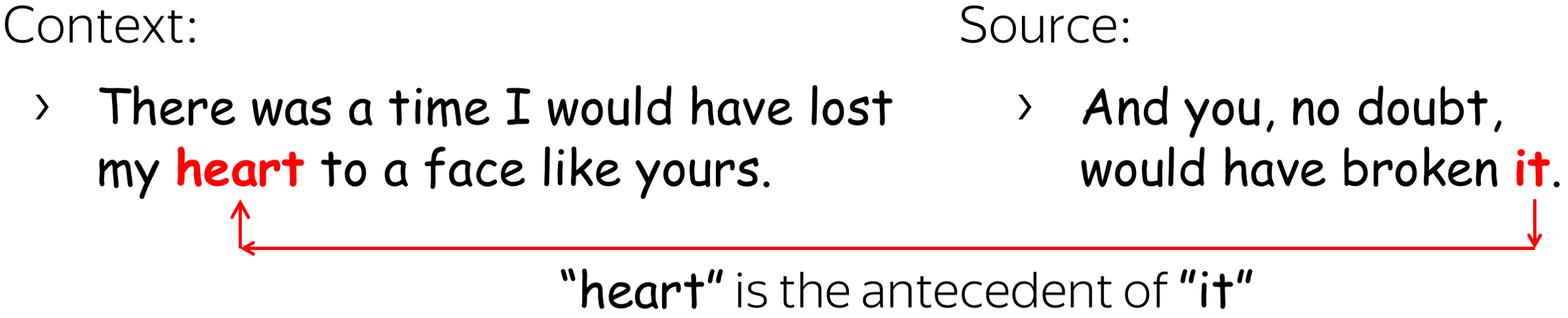
There's an ambiguous pronoun "it" in the source sentence, which refers to the "heart" in the preceding sentence.
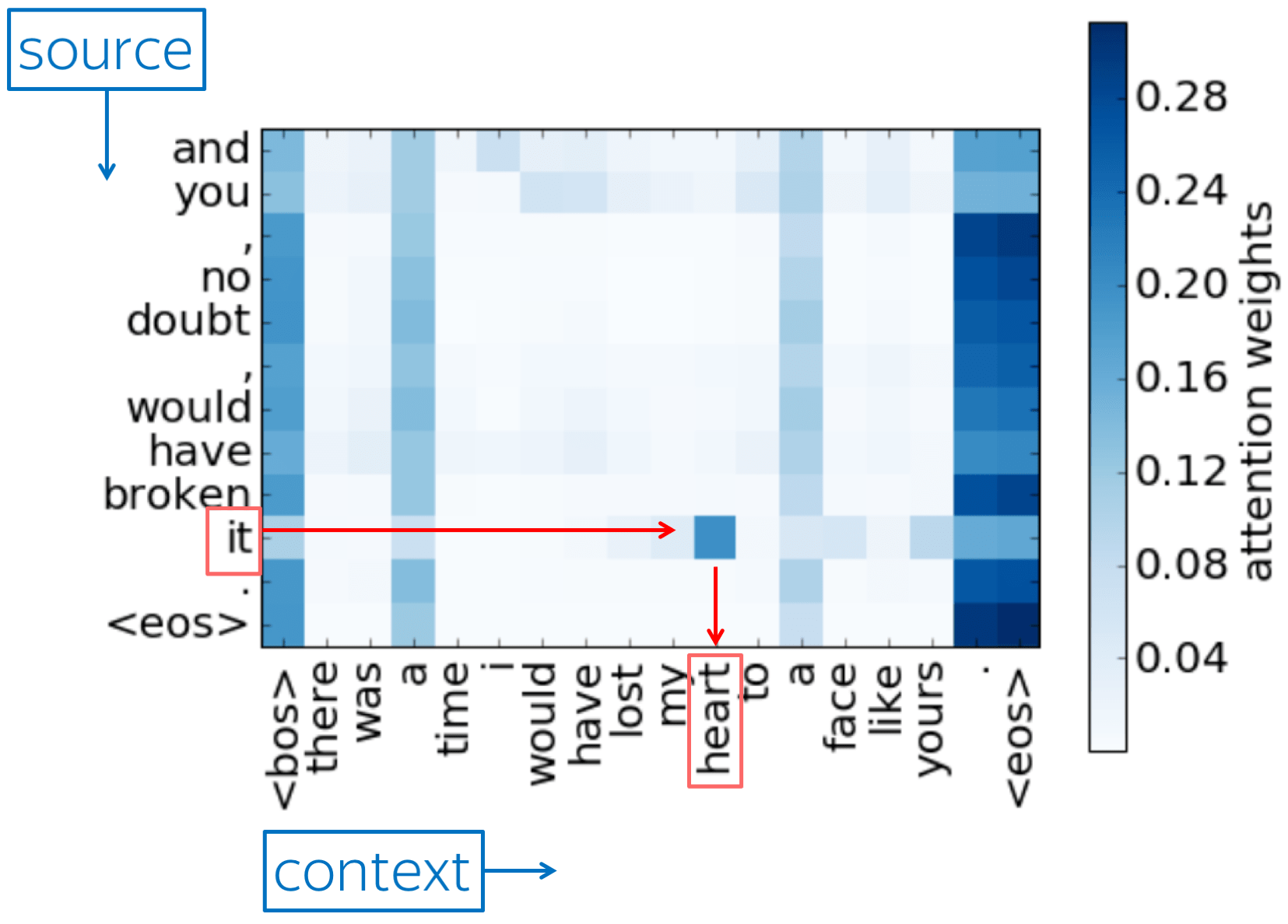
The heatmap shows which context words the model used for each source word. On the x-axis is the context sentence and on the y-axis is the source sentence.
If we look at the ambiguous pronoun "it" in the source sentence, we will see that it takes information from the noun it refers to: the "heart". We show that this is a general pattern: the model learned to identify nouns these ambiguous pronouns refer to, i.e. it learned to resolve anaphora.
Traditional vs Neural Mindsets: Dealing with Features
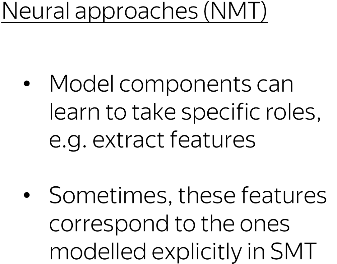
What is important: while traditional approaches engineered special-purpose features to handle various phenomena, in neural models, some components can learn to take specific roles (e.g., roles of extracting specific features). Sometimes, these features are the ones that used to be modelled explicitly in SMT (for example, anaphora). Note that this happened without any specific supervision, except for the translation task.
If we come back to our sketch, in SMT, humans used to tell models “Hey, this feature is good for you - take it!” But in NMT, a model learned to translate well, and we are again confused about how it did this. Of course, this is hard for us to fully understand how neural networks work, but as a consolation prize, we get to see that there is a specific model component that learned to extract a feature that previously, in SMT, was put into a model explicitly.
The Roles of Attention Heads in Multi-Head Self-Attention
Lena: This part is based on our ACL 2019 paper Analyzing Multi-Head Self-Attention: Specialized Heads Do the Heavy Lifting, the Rest Can Be Pruned.
Okay, we just saw that model components can be interpretable. But that model was constructed in a way that we knew where to look: we made interaction with context limited to be able to analyze it.
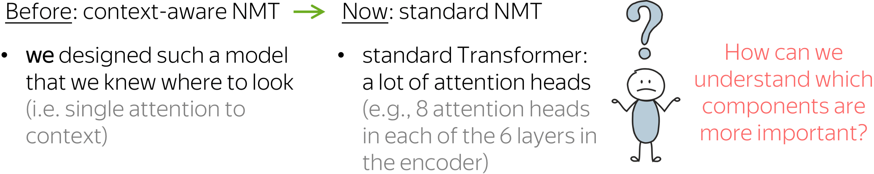
But what about standard machine translation models, for example Transformer? These models have a lot of layers and a lot of components in each layer. For example, a typical encoder has 48 attention heads! How can we understand which of them are more important?
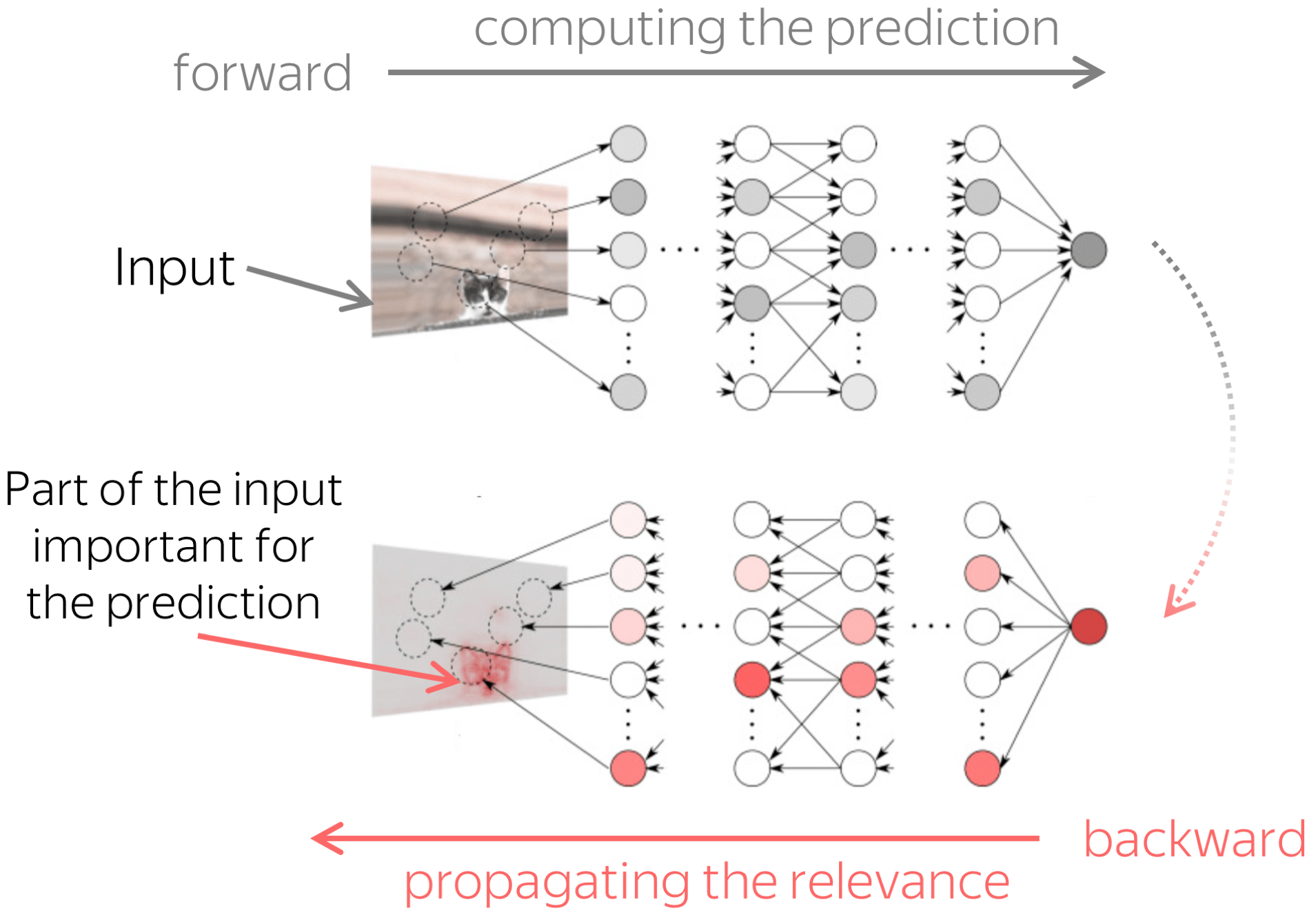
The figure is adapted from the one taken from
Dan Shiebler's blog post.
Here we took an idea from computer vision, where there are methods that propagate prediction to pixels in an input image to find parts of the image that contributed to the prediction.
We will also propagate predictions through the network. But we will do it differently from computer vision methods:
- propagate till model components (e.g., attention heads) and not till input,
- compute importance on average over a dataset and not for a single prediction.
Then we ask: on average over all predictions, which components contribute to predictions more? This is how we get the importance of attention heads. Look at the illustration of this process.
What we found is that there are only a few heads that are important. If we look at these important attention heads, surprisingly we will see that they play interpretable roles, for example, some are responsible for syntactic relations in a sentence. Below are examples of the important attention heads.
Positional heads
Model trained on WMT EN-DE
Model trained on WMT EN-DE
Model trained on WMT EN-FR
Model trained on WMT EN-FR
Model trained on WMT EN-RU
Model trained on WMT EN-RU
Model trained on OpenSubtitles EN-RU
Model trained on OpenSubtitles EN-RU
Syntactic heads
subject-> verb
verb -> subject
subject-> verb
verb -> subject
verb -> subject
object -> verb
verb -> object
object -> verb
Rare tokens head
Model trained on WMT EN-DE
Model trained on WMT EN-DE
Model trained on WMT EN-DE
Model trained on WMT EN-FR
Model trained on WMT EN-FR
Model trained on WMT EN-FR
Model trained on WMT EN-RU
Model trained on WMT EN-RU
Model trained on WMT EN-RU
Model trained on WMT EN-RU
Model trained on OpenSubtitles EN-RU
Model trained on OpenSubtitles EN-RU
Model trained on OpenSubtitles EN-RU
Here we are, again
And we are again here: the model used some of its components to represent those features that previously were given to a model explicitly, in this case, syntax.
Why is this important?
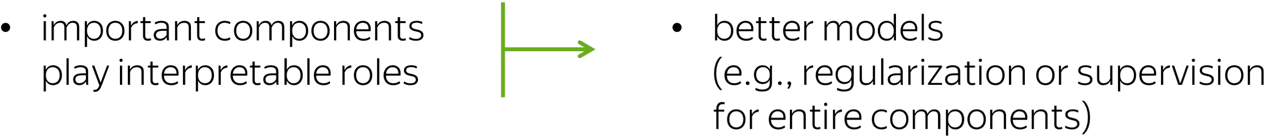
Turns out, such analysis of model components (e.g., attention heads) can also be useful. For example, it can lead to simpler models, for example with fixed attention heads that perform simple functions. Or, it can lead to better models through regularization or supervision of some components.

(Raganato et al, 2020; You et al, 2020; Tay et al, 2020 among others)
(Fan et al, 2020; Zhou et al, 2020; Peng et al, 2020 among others)
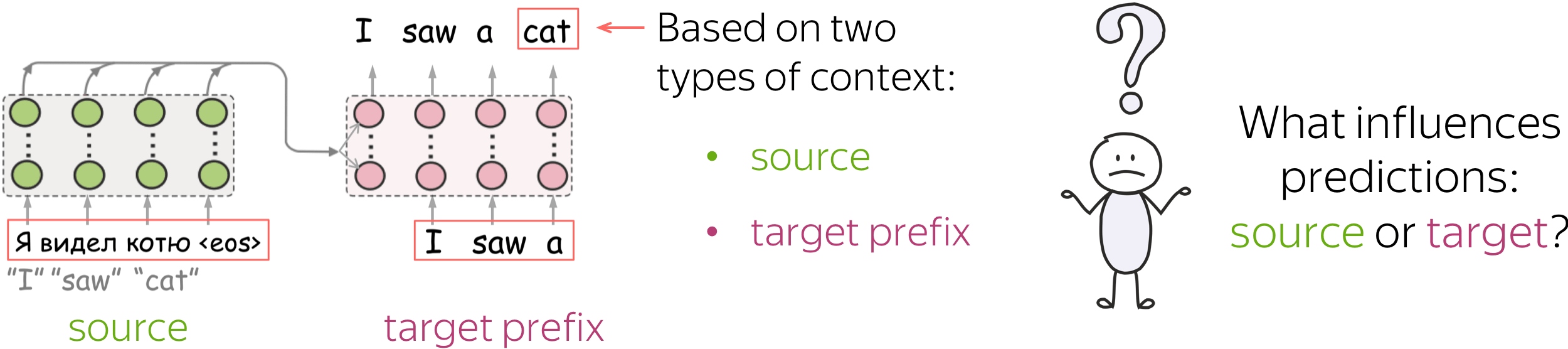
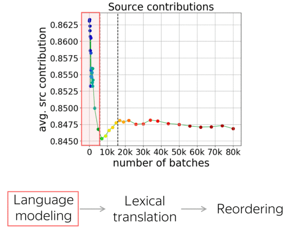
Source and Target Contributions to NMT Predictions
Lena: This part is based on our ACL 2021 paper Analyzing the Source and Target Contributions to Predictions in Neural Machine Translation.
We just looked at model components and found that sometimes they are related to SMT features. Now, let us talk about something more global: fluency and adequacy. Fluency is agreement on the target side, adequacy - connection to the source.

In traditional models, these were modelled separately: with a target-side language model (responsible for using information from the target prefix) and a translation model (responsible for using information from the source). They were trained separately, then put together. But standard neural models have to learn how to do this at once, within a single neural network.
Here our question is:
How does NMT balance being fluent (target-side LM) and adequate (translation model)?
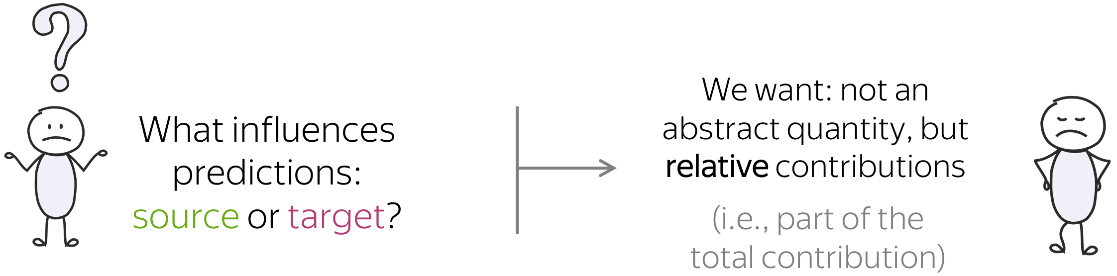
What Influences the Predictions: Source or Target?
Let me put it a bit differently. In neural machine translation, each prediction is based on two different types of context: prefix of the target sentence (i.e. previously generated tokens) and the source sentence. But it is not clear how NMT uses these types of context and what influences the predictions: source or target. Recall that in SMT, the source and the prefix were used by separate models.
In this part, we will try to understand how NMT balances these two different types of context. But first, let's think about why we care about the source-target trade-off.
Why do we care: Hallucinations and beyond.
TL;DR: Models often fail to properly use these two kinds of information.


The main reason for investigating the source-target trade-off is that NMT models often fail to properly use these two kinds of information. For example, context gates (which learn to weight source and target contexts) help for both RNNs and Transformers.
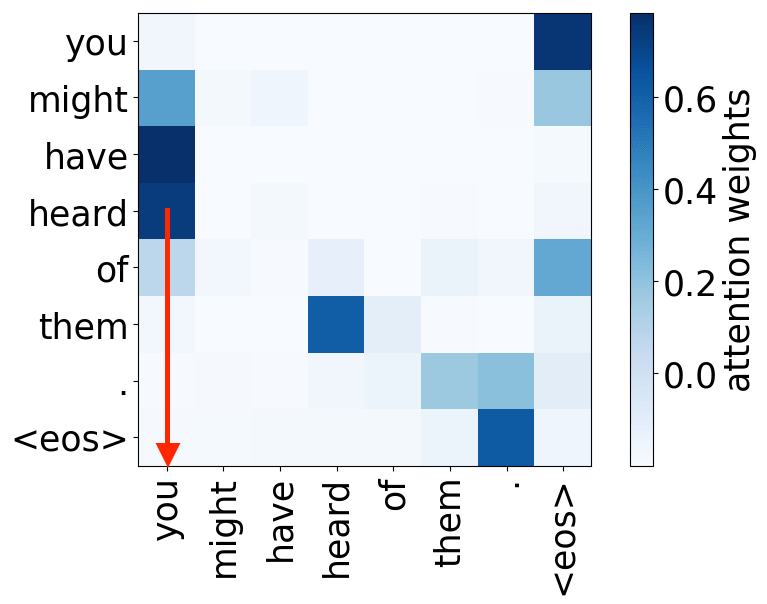
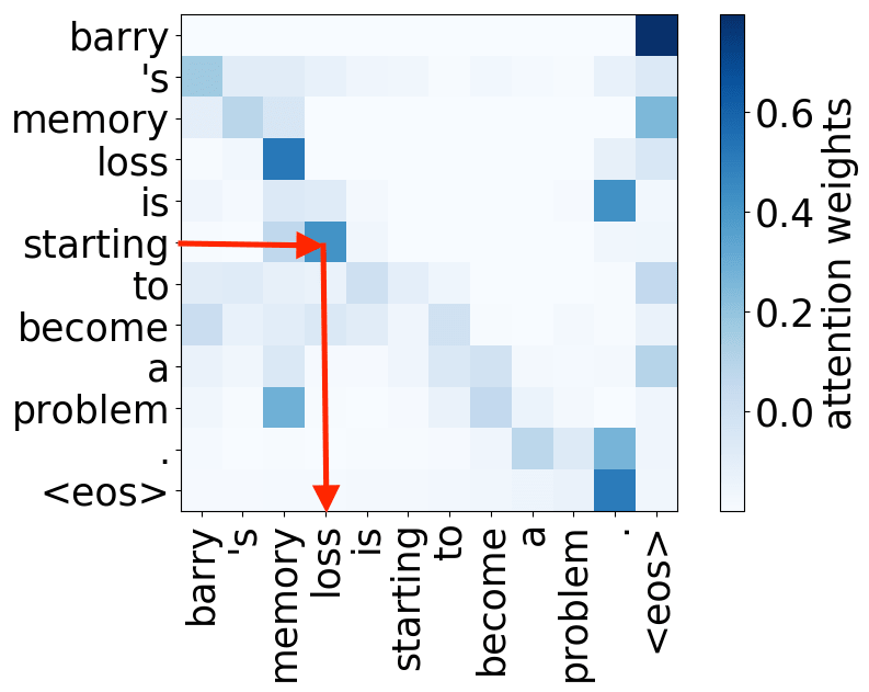
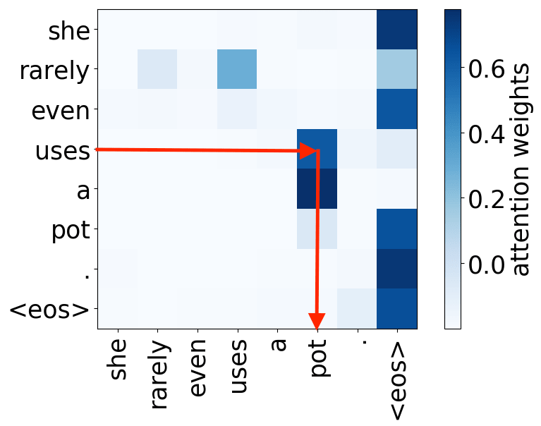
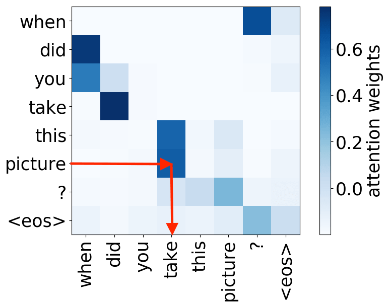
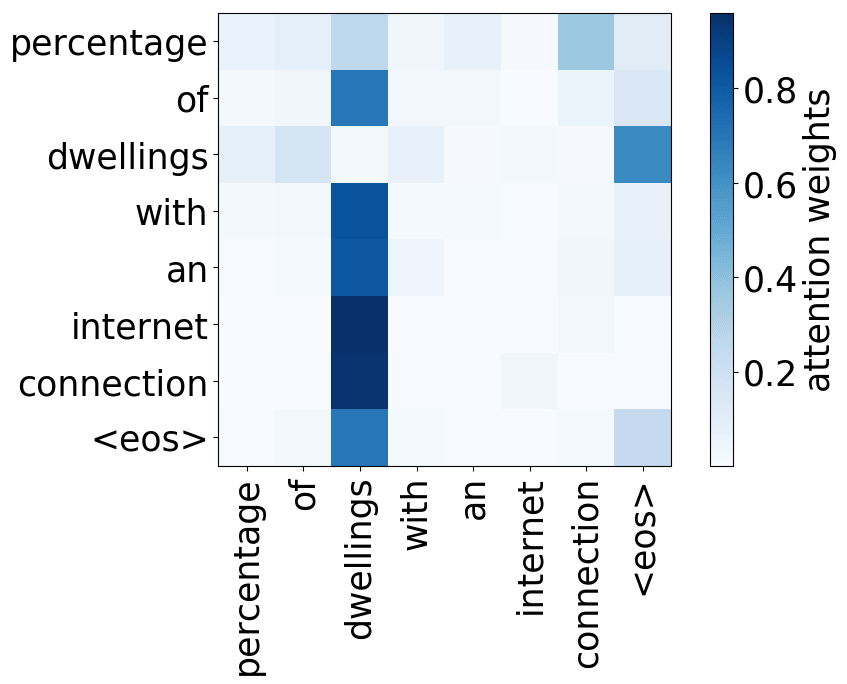
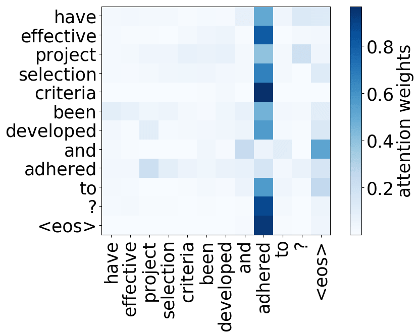
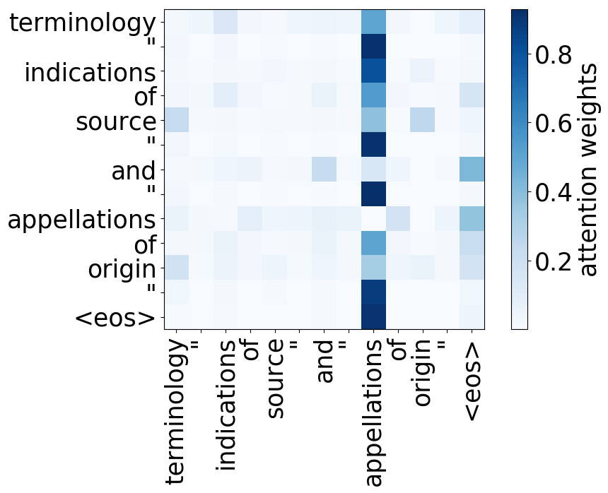
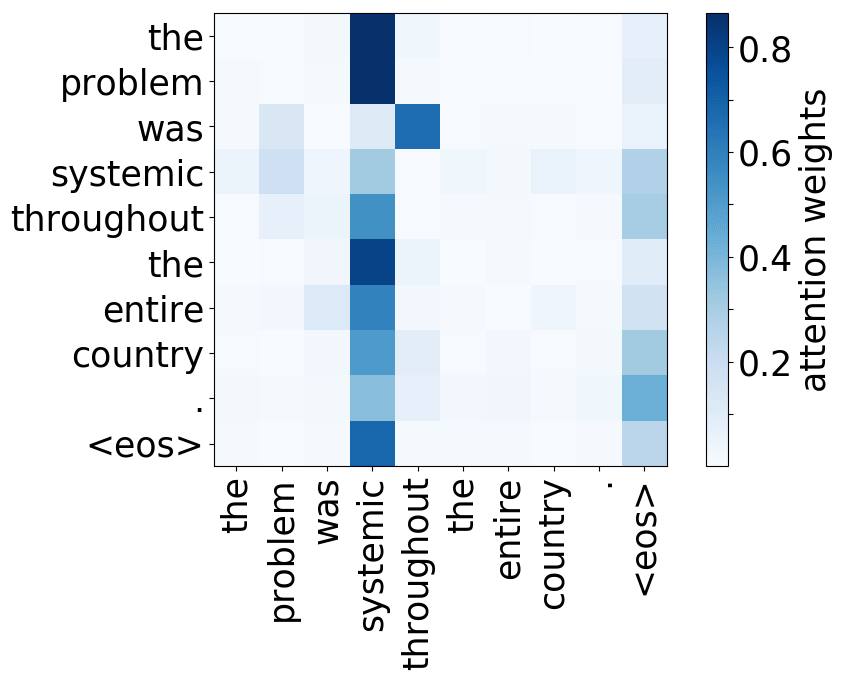
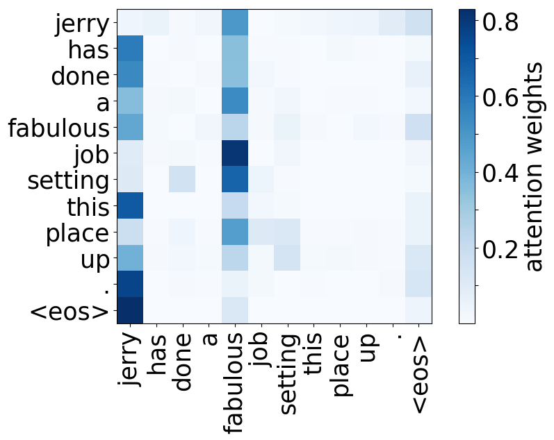
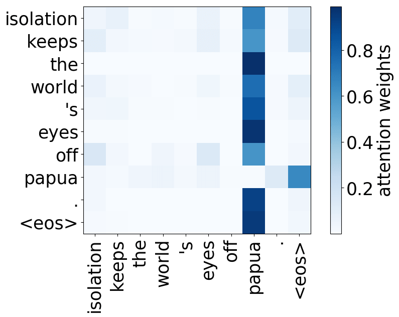
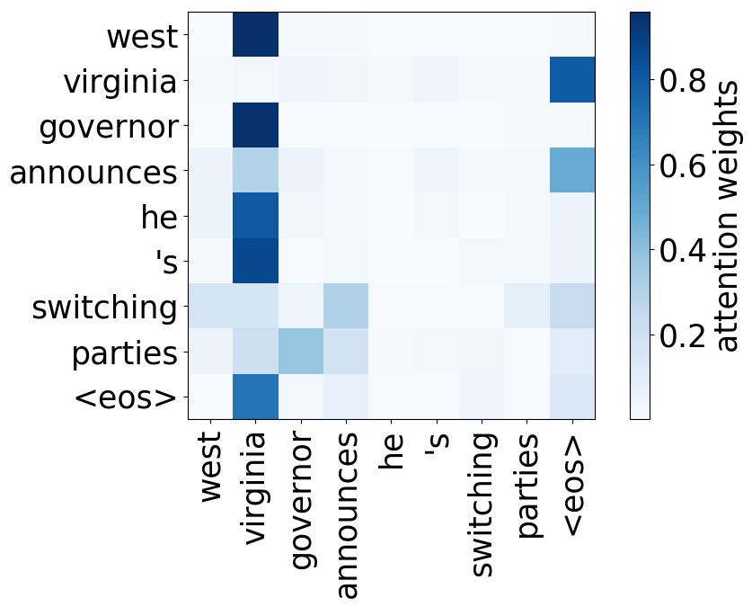
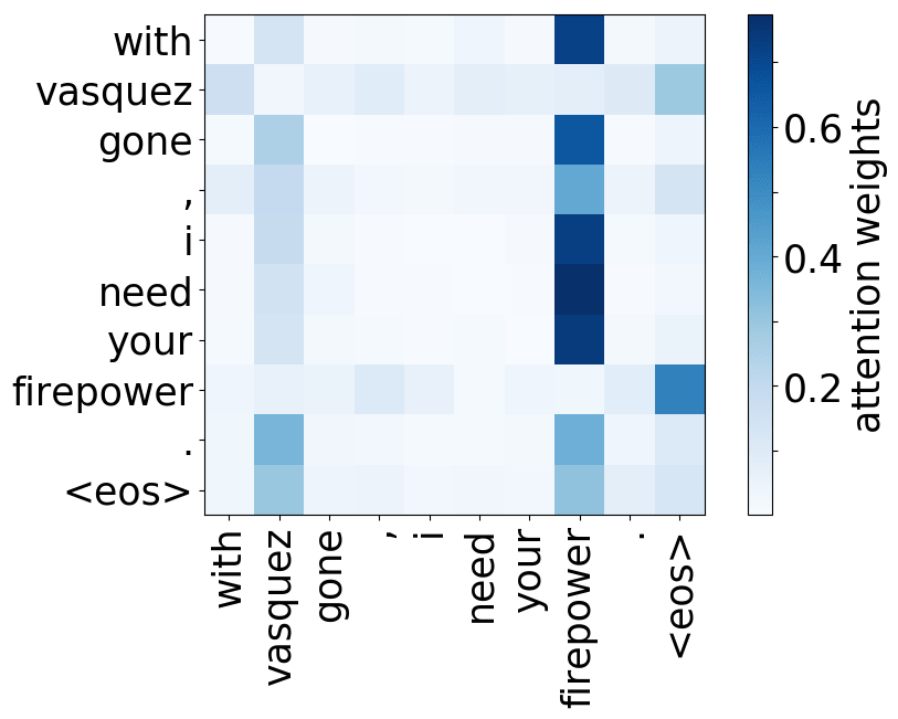
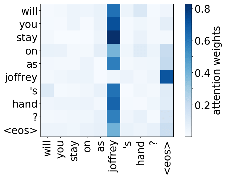
A more popular and clear example is hallucinations, when a model produces sentences that are fluent but unrelated to the source. The hypothesis is that in this mode, a model ignores information from the source and samples from its language model. While we do not know what forces a model to hallucinate in general, previous work showed some anecdotal evidence that when hallucinating, a model does fail to use source properly. Look at the examples of attention maps of hallucinating models: models may put most of the decoder-encoder attention to uninformative source tokens, e.g. EOS and punctuation.
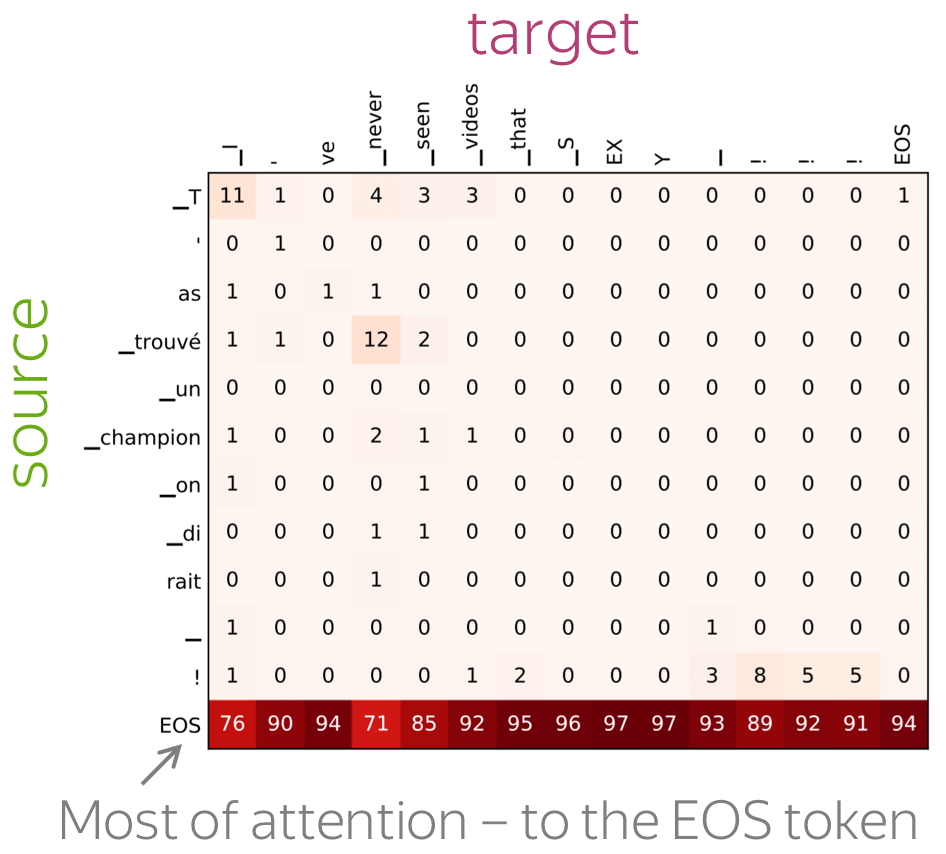
The figure is from
Berard et al, 2019.
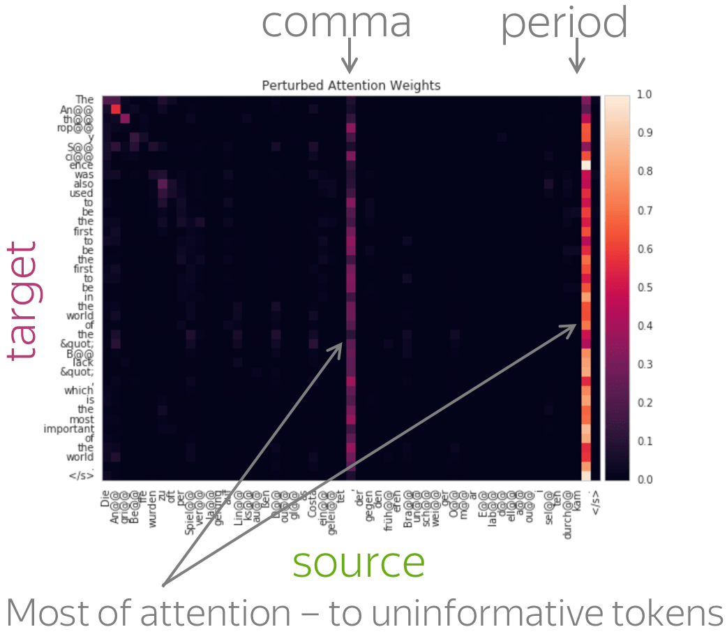
The figure is from
Lee et al, 2018.
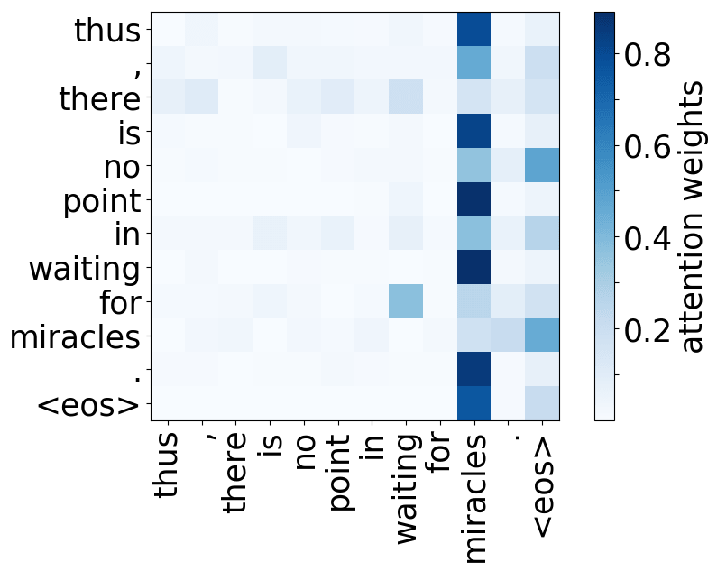
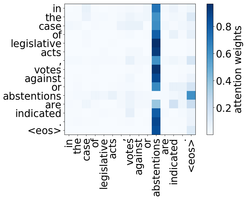
While these examples are interesting, note that this evidence is rather anecdotal: these are only a couple of examples when a model is "caught in action" and even for the same Transformer model, researchers found different patterns.
If we knew how to evaluate the source and target contributions to NMT prediction, this could be useful to evaluate techniques that force a model to rely on the source more (for example, different kinds of regularizations or training objectives) and it could help in other tasks where reliance on source is important.
We want: Relative Contributions of Source and Target
The figure is adapted from the one taken from
Dan Shiebler's blog post.
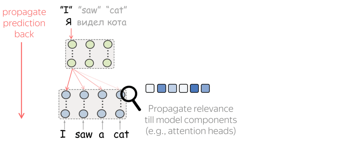
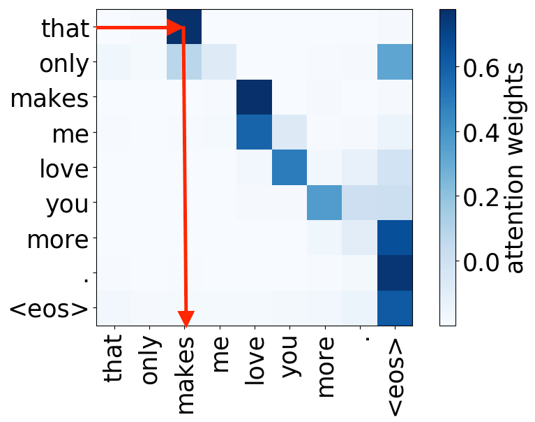
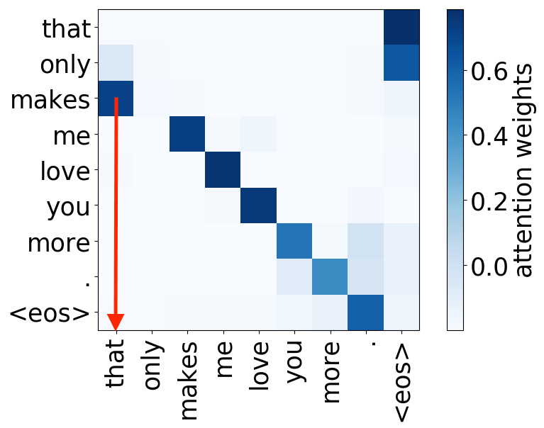
Let us come back to what we want. We want to understand what influences NMT predictions: source or target. Specifically, we want to evaluate their relative contributions. Intuitively, imagine we have everything that takes part in forming a prediction - let's call it "the total contribution". What we are interested in is part in the total contribution.
I’m not going to explain our method in detail here (for this - look at the paper), but I’ll just give you an intuitive explanation. It is a variation of the same attribution method we already used to evaluate the importance of different attention heads. We also propagate a prediction back from output to input to identify input parts that contribute to the prediction.
Intuition: Relative Token Contributions
Look at the illustration for NMT. We have a prediction, propagate it back and end up with token contributions; their total contribution equals to the prediction we propagate. Without loss of generality, we can assume that the total contribution is always 1 and we can evaluate relative token contributions.
For different generation steps, we are likely to see that the trade-off between source and target changes from token to token. Of course, for the first token source contribution is always 1 (because there is no prefix yet), but during generation, this changes.
We Look at: Total Contribution and Entropy of Contributions
We look at token contributions for each generation step separately. In this way, we'll be able to see what happens during the generation process.
• total source contribution
The total contribution of the source is the sum of contributions of source tokens. Note that since we evaluate relative contributions, \(contr(source) = 1 - contr(prefix)\).
• entropy of contributions
The entropy of contributions tells us how 'focused' the contributions are: whether the model is confident in the choice of relevant tokens or spreads its relevance across the whole input. In this talk (blog post), we will mostly see the total source contribution, but in the paper, we also consider the entropy of source and target contributions.
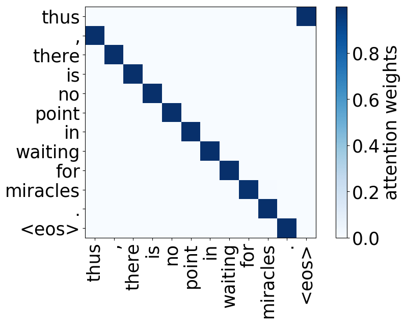
Source Contribution to Different Target Positions
We are mainly interested not in the absolute values of contributions, but in how these patterns change depending on data, training objective, or timestep in training. But first, let’s look at the source contribution for a single model.
• source contribution: decreases during generation
For each target position, the figure shows the source contribution. We see that, as the generation progresses, the influence of source decreases (i.e., the influence of target increases). This is expected: with a longer prefix, it becomes easier for the model to understand which source tokens to use, and at the same time, it needs to be more careful to generate tokens that agree with the prefix.
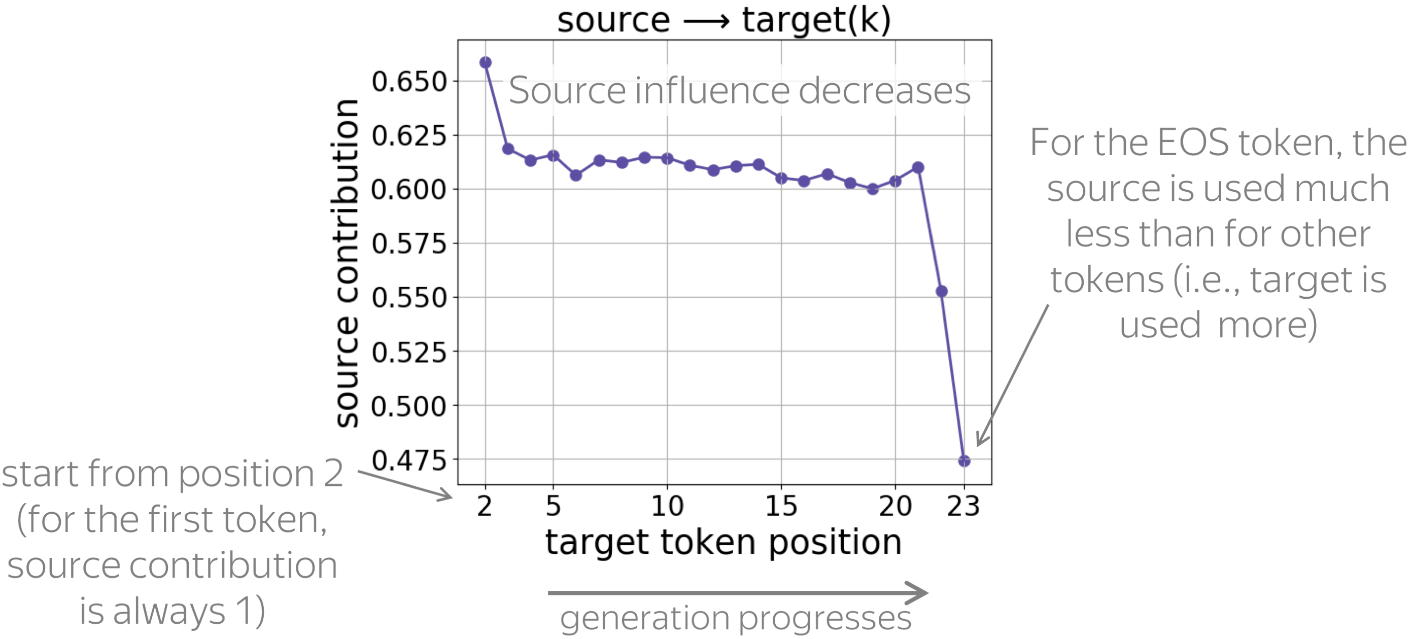
Note also a large drop of source influence for the last token: apparently, to generate the EOS token, the model relies on prefix much more than when generating other tokens.
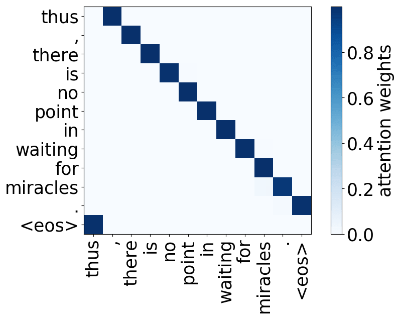
Reference, Model and Random Prefixes
Now, let us look at the changes in these patterns when conditioning on different types of target prefixes: reference, model translations, and prefixes of random sentences.
• model-generated prefixes: the simpler ones
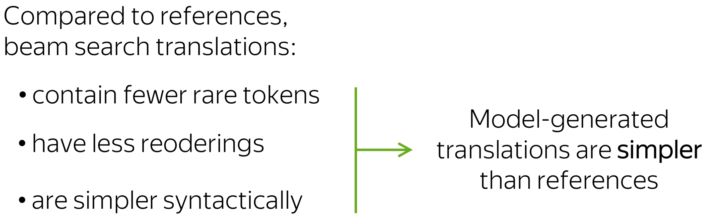
First, let us compare how models react to prefixes that come from reference and model translations. We know that beam search translations are usually simpler than references: several papers show that they contain fewer rare tokens, have fewer reorderings, and are simpler syntactically.
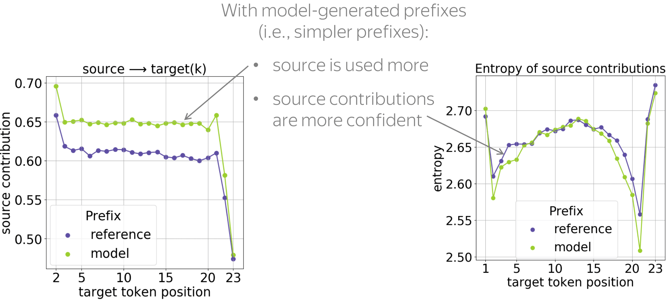
When conditioned on these simpler prefixes, the model relies on the source more and is more confident when choosing relevant source tokens (the entropy of source contributions is lower). We hypothesize that these simpler prefixes are more convenient for the model, and they require less reasoning on the target side.
• random prefixes: the unexpected ones
Now, let us give a model something unexpected: prefixes of random sentences. In this experiment, a model has a source sentence and a prefix of the target sentence, which do not make sense together.
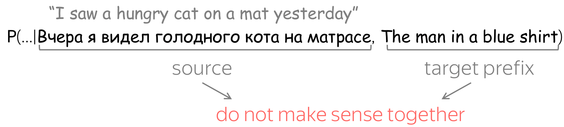
Why random prefixes?
We are interested in this setting, because
- we want to understand what happens when a model is hallucinating;
- a random prefixe is a simple way to simulate hallucination mode.
What will our model do?
Our model is given source and prefix which do not make sense together. What will it do? Previous work tells us that, in principle, NMT models can ignore the source: this is when they fall into hallucination mode. On the other hand, another work studied exposure bias and showed that language models have the self-recovery ability: when a model is given a gibberish prefix, it ignores it and continues to generate reasonable things.
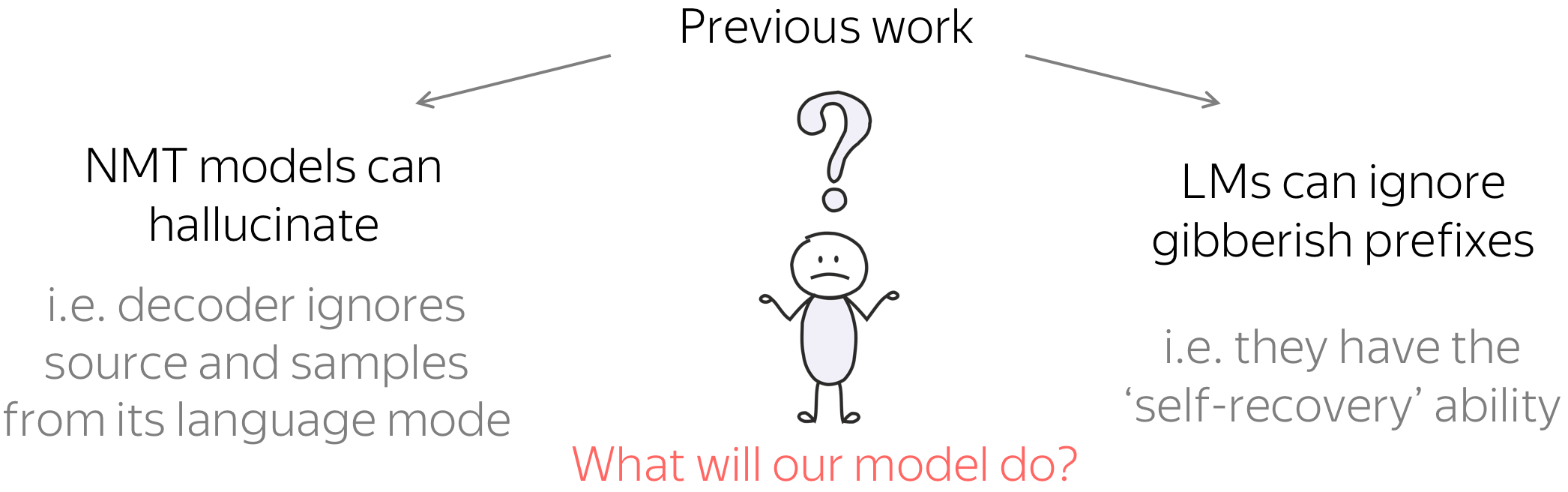
What will our model do: ignore the source or the prefix? Previous work shows that, in principle, our model can ignore either the source or the prefix.
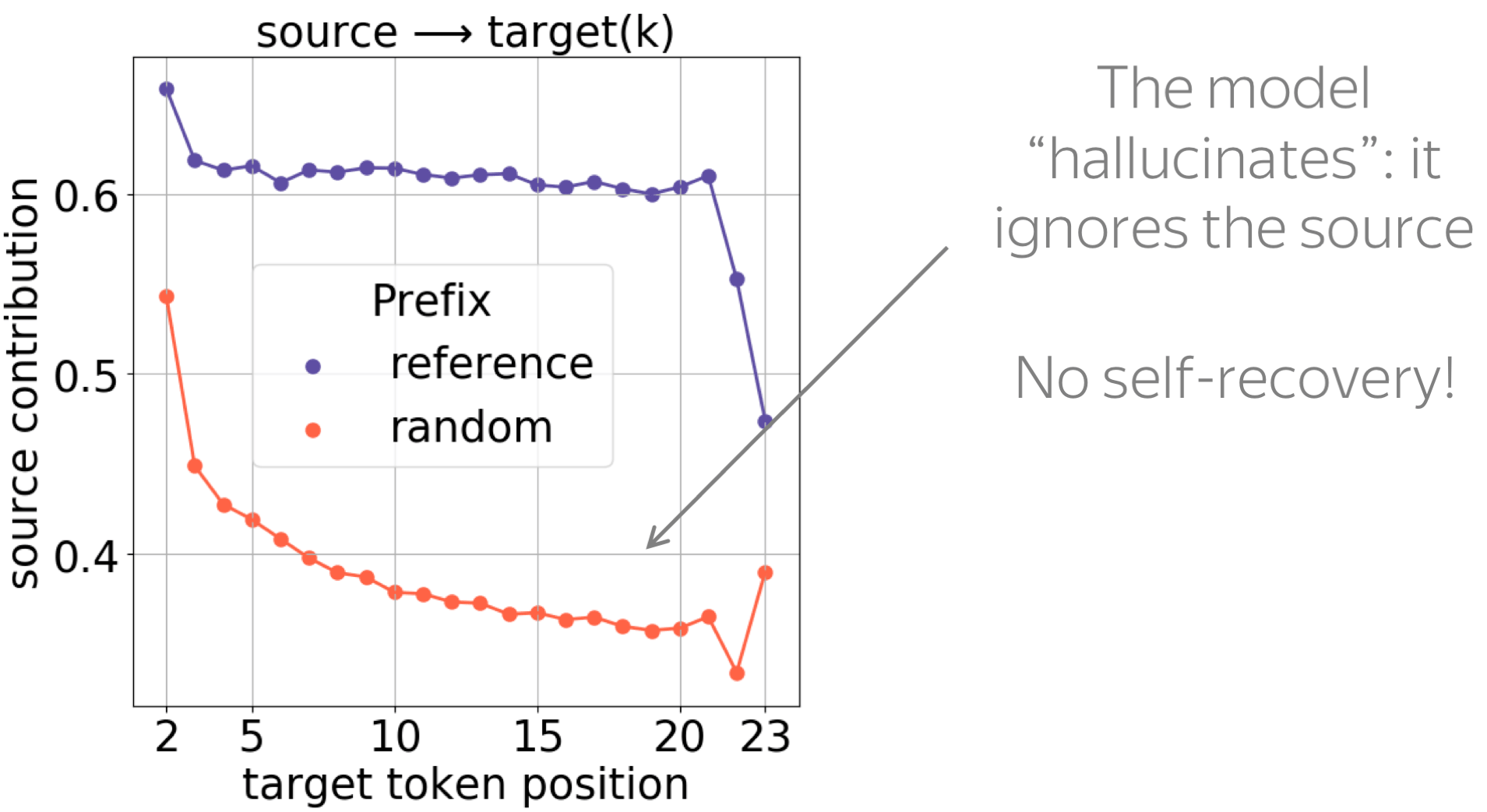
As we see from the results, the model tends to fall into hallucination mode even when a random prefix is very short, e.g. one token: we see a large drop of source influence for all positions. This behavior is what we would expect when a model is hallucinating, and there is no self-recovery ability.
Exposure Bias and Source Contributions
The results we just saw agree with some observations made in previous work studying self-recovery and hallucinations. Now, we illustrate more explicitly how our methodology can be used to shed light on the effects of exposure bias and training objectives.
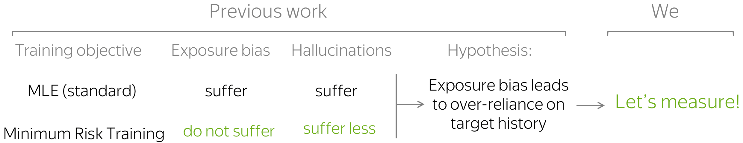
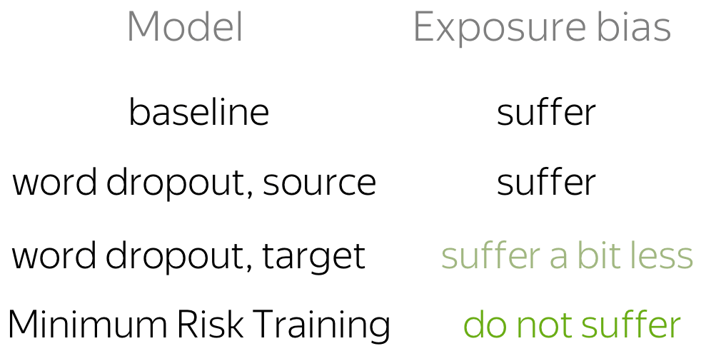
Exposure bias means that in training, a model sees only gold prefixes, but at test time, it uses model-generated prefixes (which can contain errors). This ACL 2020 paper suggests that there is a connection between the hallucination mode and exposure bias: the authors show that Minimum Risk Training (MRT), which does not suffer from exposure bias, reduces hallucinations. However, they did not directly measure the over-reliance on target history. Luckily, now we can do this :)
How: Feed Different Prefixes, Look at Contributions
We want to check to what extent models that suffer from exposure bias to differing extent are prone to hallucinations. For this, we feed different types of prefixes, prefixes of either model-generated translations or random sentences, and look at model behavior. While conditioning on model-generated prefixes shows what happens in the standard setting at model's inference, random prefixes (fluent but unrelated to source prefixes) show whether the model is likely to fall into a language modeling regime, i.e., to what extent it ignores the source and hallucinates.
In addition to the baseline and the models trained with the Minimum Risk Training objective (considered in previous work), we also experiment with word dropout. This is a data augmentation method: in training, part of tokens are replaced with random. When used on the target side, it may serve as the simplest way to alleviate exposure bias: it exposes a model to something other than gold prefixes. This is not true when used on the source side, but for analysis, we consider both variants.
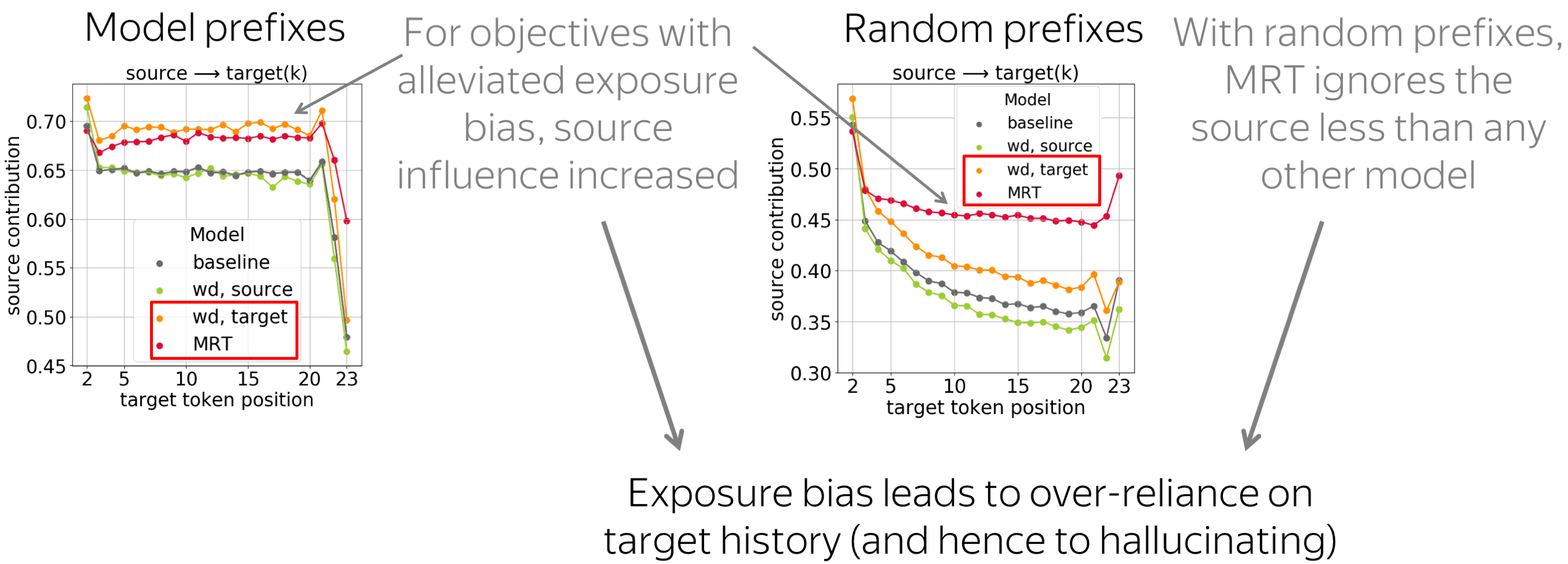
The results for both types of prefixes confirm our hypothesis:
Models suffering from exposure bias are more prone to over-relying on target history (and hence to hallucinating) than those where the exposure bias is mitigated.
Indeed, we see that MRT-trained models ignore source less than any other model; the second best for random prefixes is the target-side word dropout, which also reduces exposure bias.
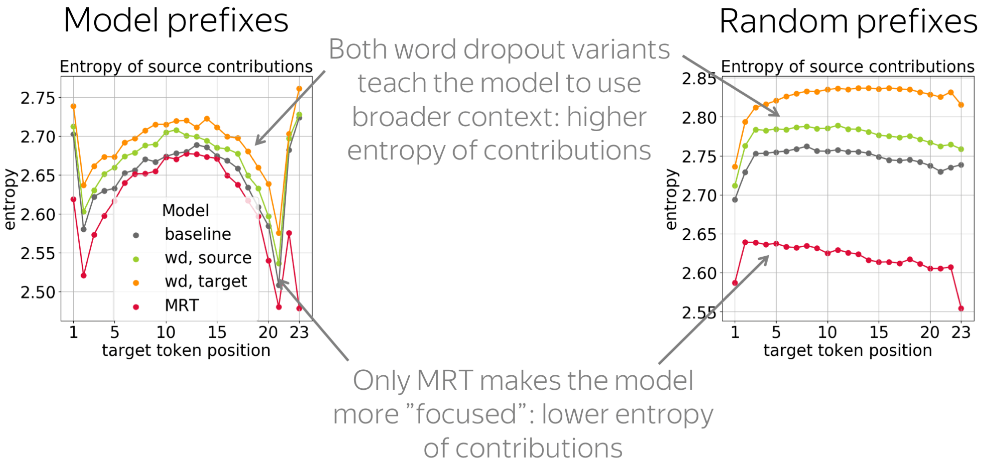
It is also interesting to look at the entropy of source contributions to see whether these objectives make the model more or less "focused". We see that only MRT leads to more confident contributions of source tokens: the entropy is lower. In contrast, both word dropout variants teach the model to use broader context.
More in the paper:
Varying the Amount of Data
- Models trained with more data use source more and do it more confidently
For more details on this, see the paper or its blog post.
Training Process: Non-Monotonic with Several Distinct Stages
Finally, we look at what happens during model training. For model checkpoints during training, we look at the changes in the contribution patterns.
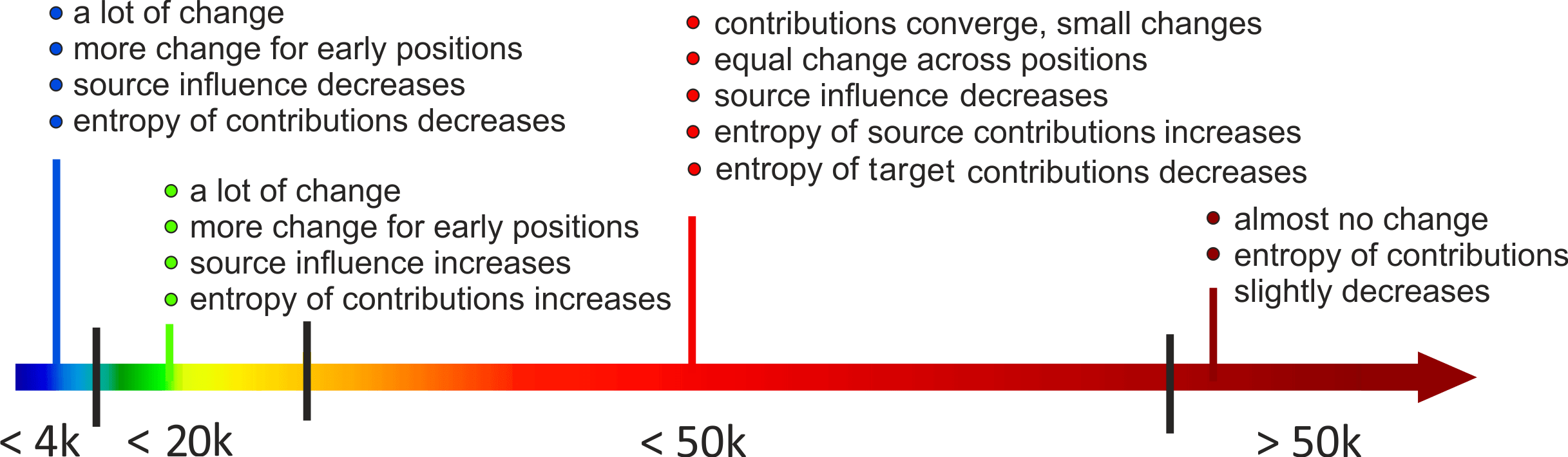
In the paper, we have a lot of experiments and we end up with such a training pipeline: it shows what happens during each stage of the training (on the x-axis is the number of training batches). For more details on this pipeline, look at the paper. Here I’ll mention only the results we need for the next part.
• changes in contributions are non-monotonic
These figures show how the total contribution of source and the entropy of source contributions change during training. On the x-axis is the training step, and the graph shows average over target positions and examples.
We see that the changes are not monotonic: first source contribution goes down, then up, then little is going on. For the entropy of contributions, the behavior is the same. Overall, the changes during training are not monotonic, which means that NMT training has several stages with qualitatively different changes.
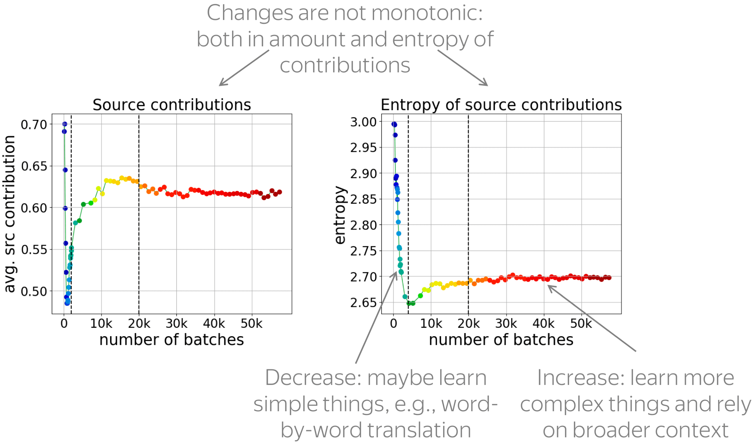
We hypothesize that when the entropy of contributions decreases, the model learns simple patterns, for example, word-by-word translation. When source contribution and its entropy do up, we think that the model starts to rely on a broader context and learns more complicated things.
So far, we just hypothesize that this is what happens. But what is really going on? Let's find out.
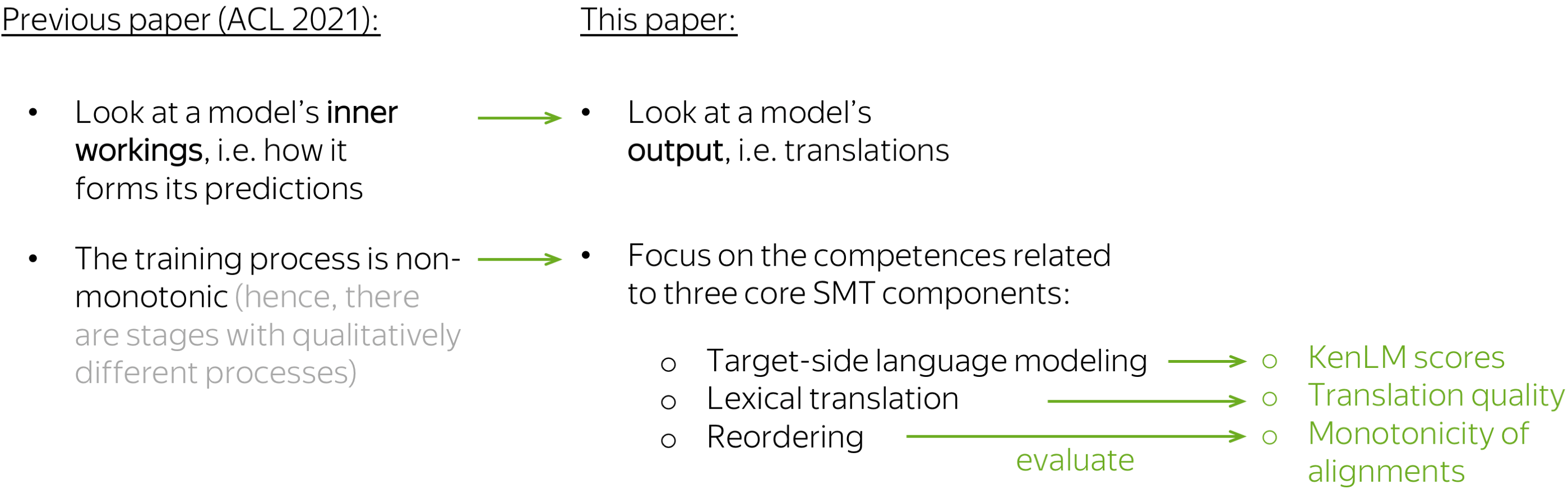
NMT Training through the Lens of Classical SMT
Lena: This part is based on the OpenReview paper Language Modeling, Lexical Translation, Reordering: The Training Process of NMT through the Lens of Classical SMT.
Let us recall that classical SMT splits the translation task into several components corresponding to the competences which researchers think the model should have. The typical components are: target-side language model, lexical translation model, and a reordering model. Overall, in SMT different competences are modelled with distinct model components which are trained separately and then put together.

In NMT, the whole translation task is modelled with a single neural network. And the question is:
How does NMT acquire different competences during training?
For example, are there any stages where NMT focuses on fluency or adequacy, or does it improve everything at the same rate? Does it learn word-by-word translation first and more complicated patterns later, or is there a different behavior?
This is especially interesting in light of our ACL 2021 paper we just discussed. There we looked at a model’s inner working (namely, how the predictions are formed) and we saw that the training process is non-monotonic, which means that there are stages with qualitatively different changes. This other paper looks at the model’s output and focuses on the competences related to three core SMT components: target-side language modeling, lexical translation, and reordering.
Target-Side Language Modeling
Let’s start with the language modeling scores. Here the x-axis shows the training step. We see that most of the change happens at the beginning of training. Also, the scores peak much higher than that of references (shown with the dashed line here). This means that the model probably generates very frequent n-grams rather than diverse texts similar to references.
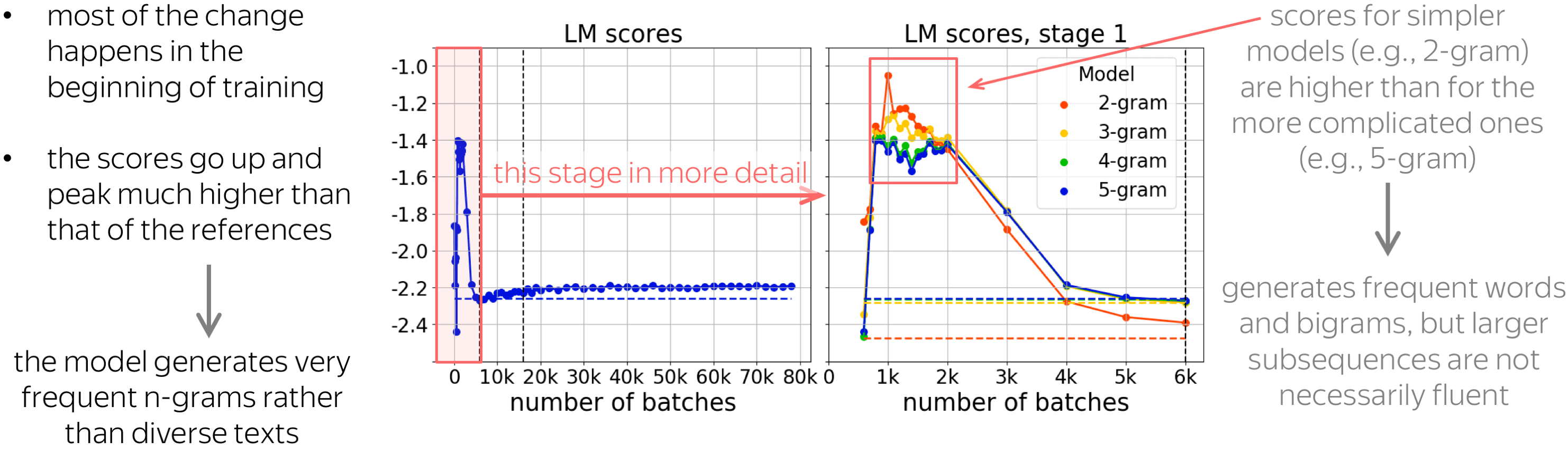
Let’s look at this early stage more closely and consider KenLM models with different context lengths: from bigram to 5-gram models. We see that for some part of training, scores for simpler models are higher than for the more complicated ones. For example, the 2-gram score is the highest and the 5-gram score is the lowest. This means that the model generates frequent words and n-grams, but larger subsequences are not necessarily fluent.
Below is an example of how a translation evolves at this early stage. This is English-German, our source sentence is six months of construction works, that’s brutal. On the left are model translations, and on the right is their approximate version in English.
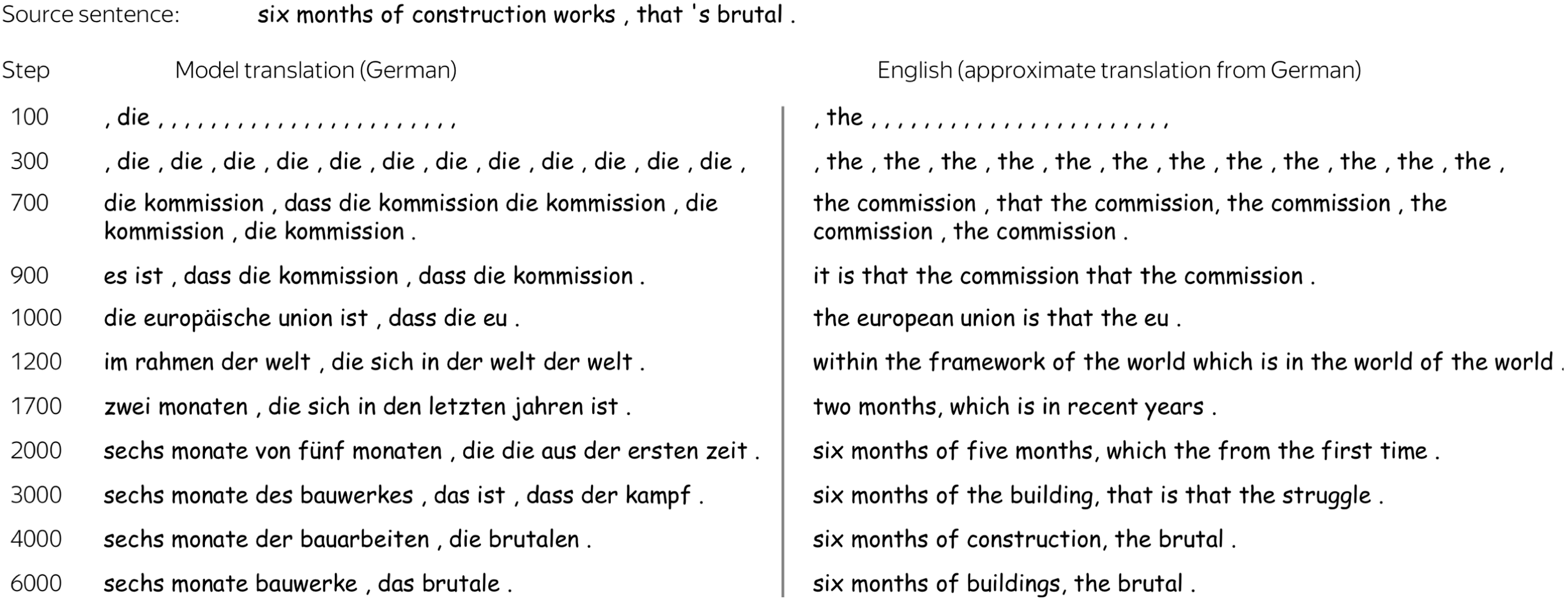
We see that first, the model hallucinates the most frequent token, then bigram, the three-gram, then combinations of frequent phrases. After that, words related to the source start to appear, and only later we see something reasonable.
Translation Quality
Let’s now turn to translation quality. In addition to the BLEU score (which is the standard automatic evaluation metric for machine translation), the paper also shows token-level accuracy for target tokens of different frequency ranks. Token-level accuracy is the proportion of cases where the correct next token is the most probable choice. Note that this is exactly what the model is trained to do: in a classification setting, it is trained to predict the next token.
We see that for rare tokens, accuracy improves slower than for the rest. This is expected: rare phenomena are learned later in training. What is not clear, is what happens during the last half of the training: changes in both BLEU and accuracy are almost invisible, even for rare tokens.
Monotonicity of Alignments
Luckily, we have one more thing to look at: monotonicity of alignments. The graph shows how the monotonicity of alignments changes during training. For more details on the metric, look at the paper, but everything we need to know now is that lower scores mean less monotonic (or more complicated) alignments in generated translations.
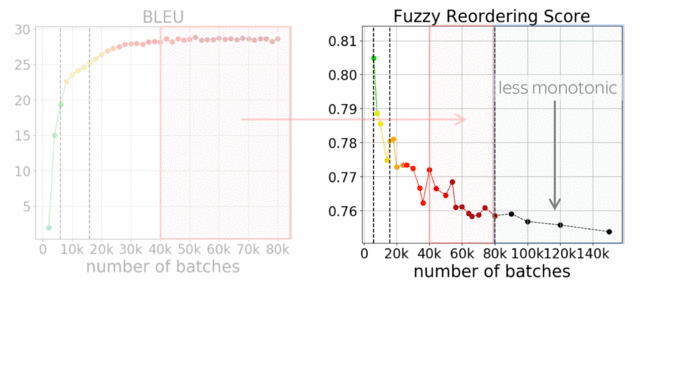
First, let's look again at the second half of the training we just looked at. While changes in quality are almost invisible, reorderings change significantly. In the absolute values this does not look like a lot, a bit later I’ll show you some examples and how this analysis can be used in practice to improve non-autoregressive NMT - you’ll see that these changes are quite prominent.
What is interesting, is that changes in the alignments are visible even after the model converges in terms of BLEU. This relates to one of our previous works on context-aware NMT (Voita et al, 2019): we observed that even after BLEU converges, discourse phenomena continue to improve.
Here are a couple of examples of how translations change during this last part of the training: the examples are for English-German and English-Russian, and same-colored chunks are approximately aligned to each other.
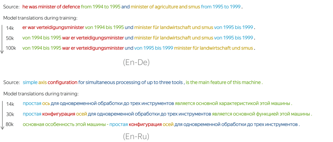
I don’t expect you to understand all the translations, but visually we can see that first, the translations are almost word-by-word, then the reordering becomes more complicated. For example, for English-Russian, the last phrase (shown in green) finally gets reordered to the beginning of the sentence. Note that the reorderings at these later training steps are more natural for the corresponding target language.
Characterizing Training Stages
Summarizing all the observations, we can say that NMT training undergoes three stages:
- target-side language modeling,
- learning how to use source and approaching word-by-word translation,
- refining translations, which is visible only by changes in the reordering and not visible by standard metrics.
Now let’s look at how these results agree with the stages we looked at in the previous paper. First, the source contribution goes down. Here the model relies on the target-side prefix and ignores the source, and looking at translations confirmed that here it learns language modeling. Then, the source contribution increases rapidly: the model starts to use the source, and we saw that the quality improves quickly. After these two stages, translations are close to word-by-word ones. Finally, where very little is going on, reorderings continue to become significantly more complicated.
Practical Applications of the Analysis
Finally, not only this is fun, but it can also be useful in practice. First, there are various settings where data complexity is important: therefore, translations from specific training stages can be useful. Next, there are a lot of SMT-inspired modeling modifications, and our analysis can help modeling modifications.


(using target-side language models, lexical tables, alignments, modeling phrases, etc.)
Links
Athur et al, 2016; He et al, 2016; Tang et al, 2016; Wang et al, 2017; Zhang et al, 2017a; Dahlmann et al, 2017; Gülçehre et al, 2015; Gülçehre et al, 2017; Stahlberg et al, 2018; Mi et al, 2016; Liu et al, 2016; Chen et al, 2016; Alkhouli et al, 2016; Alkhouli & Ney, 2017; Park & Tsvetkov, 2019; Song et al, 2020 among others
Non-Autoregressive Neural Machine Translation
The paper focuses only on the first point, and as an example considers non-autoregressive NMT. For non-autoregressive models, it is standard to use sequence-level distillation. This means that targets for these models are not references but translations from an autoregressive teacher.
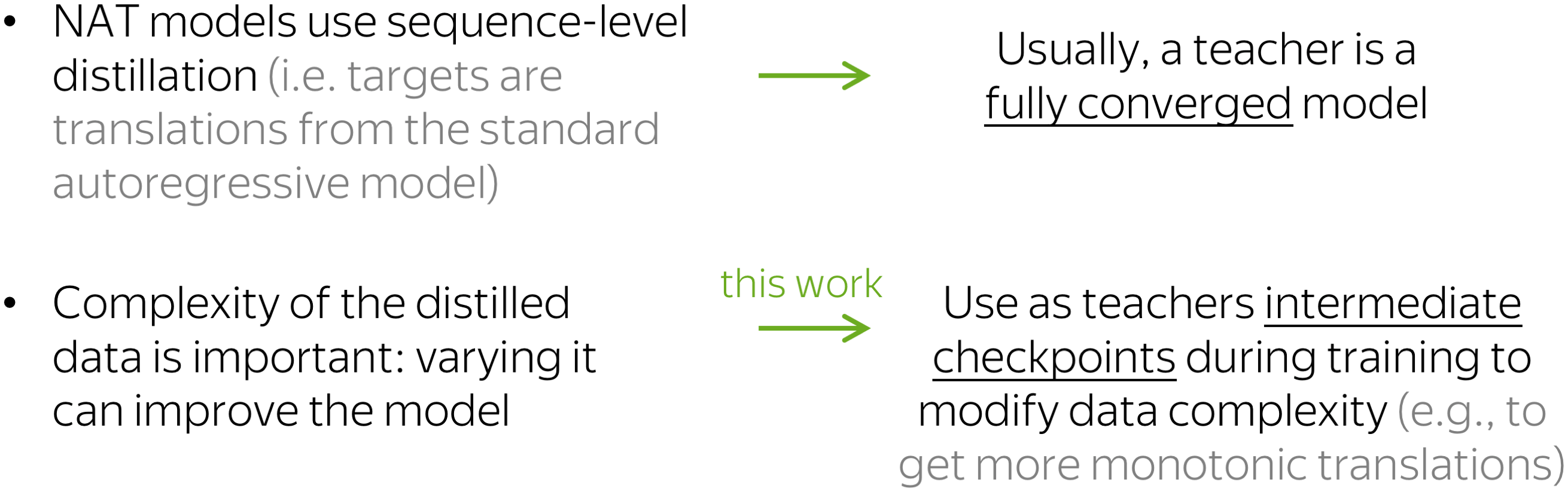
Previous work showed that complexity of the distilled data matters, and varying it can improve a model. While usually, a teacher is a fully converged model, this paper proposes to use as teachers intermediate checkpoints during model’s training to get targets of varying complexity. For example, these earlier translations have more monotonic alignments.
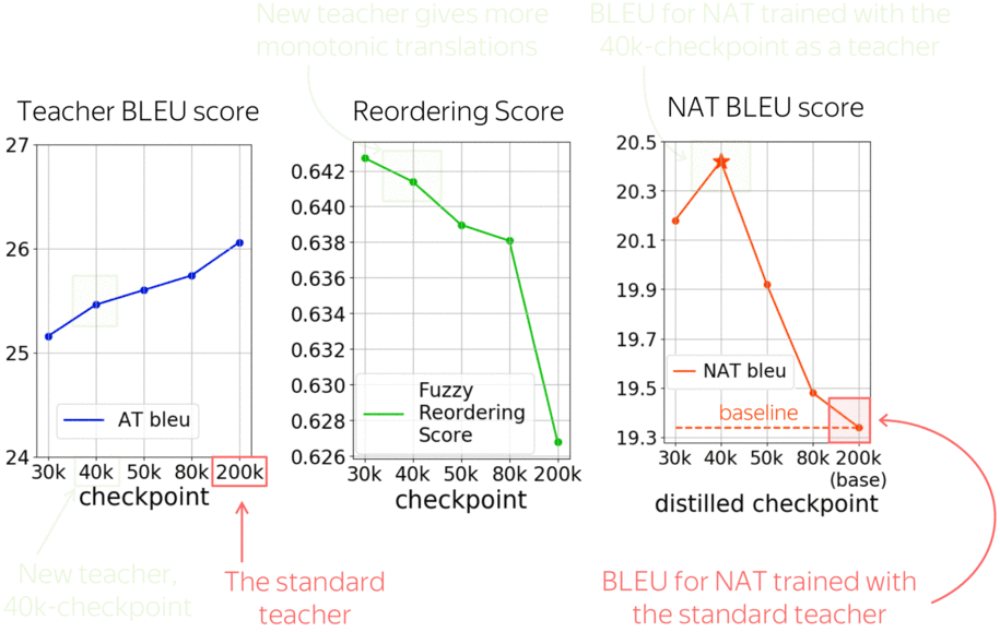
Let us look at a vanilla non-autoregressive model trained with different teachers. The standard teacher is the fully converged model, in this case after 200k training steps. But earlier checkpoints, for example after 40k-steps, have not much worse BLEU score, but significantly more monotonic alignments. And using these less trained teachers improves a vanilla NAT model by more than 1 bleu!
Takeaway
We started by noting that the two machine translation paradigms, traditional SMT and currently standard NMT, are very different conceptually. Statistical MT (SMT) decomposes the translation task into several components which are learned separately and then combined in a translation model. Differently, neural MT (NMT) models the entire translation process with a single neural network that is trained end-to-end.
In this talk, I tried to shed some light on the workings of neural MT while keeping in mind how things used to be done in SMT. We saw that:
- NMT model components can learn to extract features that were put explicitly in SMT;
- while using the prefix and the source co-exist in the same model in NMT, we can still look at how NMT does this;
- NMT training consists of the stages where it focuses on competences mirroring three core SMT components: language modeling, translation, reordering.
Want to know more?
- Context-Aware Neural Machine Translation Learns Anaphora Resolution: [paper]
- Analyzing Multi-Head Self-Attention: Specialized Heads Do the Heavy Lifting, the Rest Can Be Pruned: [paper] [blog]
- Analyzing the Source and Target Contributions to Predictions in Neural Machine Translation: [paper] [blog]
- Language Modeling, Lexical Translation, Reordering: The Training Process of NMT through the Lens of Classical SMT: [paper]
Share: Tweet