(Introduction to) Transfer Learning
Lena: Transfer Learning is huge: therefore, it is not possible to cover it all in a single lecture. Here I will try to give a general idea of transfer and will show some popular ways it is currently done.
Before the era of Large Language Models (such as e.g. ChatGPT), Transfer Learning was likely to be the most popular NLP area both in research and industry. Most probably you've already heard people talking about ELMo, BERT, and other characters - after this lecture, you will understand why!
"Transfer" Knowledge from One Model to Another
The general idea of transfer learning is to "transfer" knowledge from one task/model to another. For example, you don't have a huge amount of data for the task you are interested in (e.g., classification), and it is hard to get a good model using only this data. Instead, you can have data for some other task, which is easier to get (e.g., for language modeling you don't need labels at all - plain texts are enough).
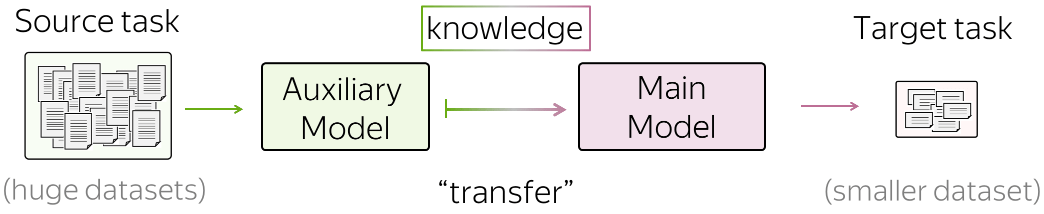
In this case, you can "transfer" knowledge from the task you are not interested in (let's call it source task) to the task you care about, i.e. target task.
A Taxonomy for Transfer Learning in NLP
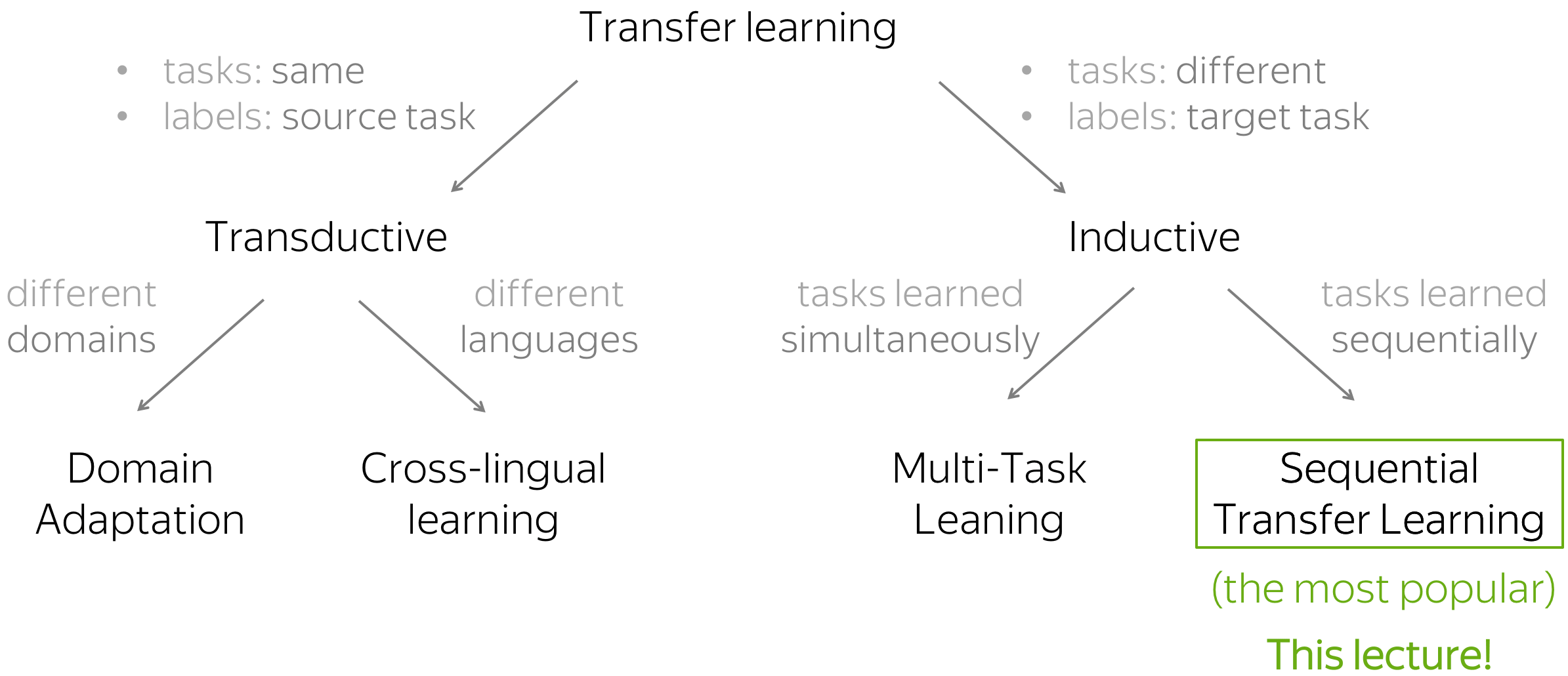
There are several types of transfer that are categorized nicely in Sebastian Ruder's blog post. Two large categories are transductive and inductive transfer learning: they divide all approaches into the ones where the task is the same and labels are only in the source (transductive), and where the tasks are different and labels are only in the target (inductive).
This taxonomy is from
Sebastian Ruder's blog post.
In this lecture, we are interested in the latter, with different tasks, and in its subcategory that learns these tasks sequentially.
Lena: I'm usually reluctant to make such claims, but here I believe it is safe to say that sequential transfer learning is currently one of the most popular areas of research.
What we'll be looking at
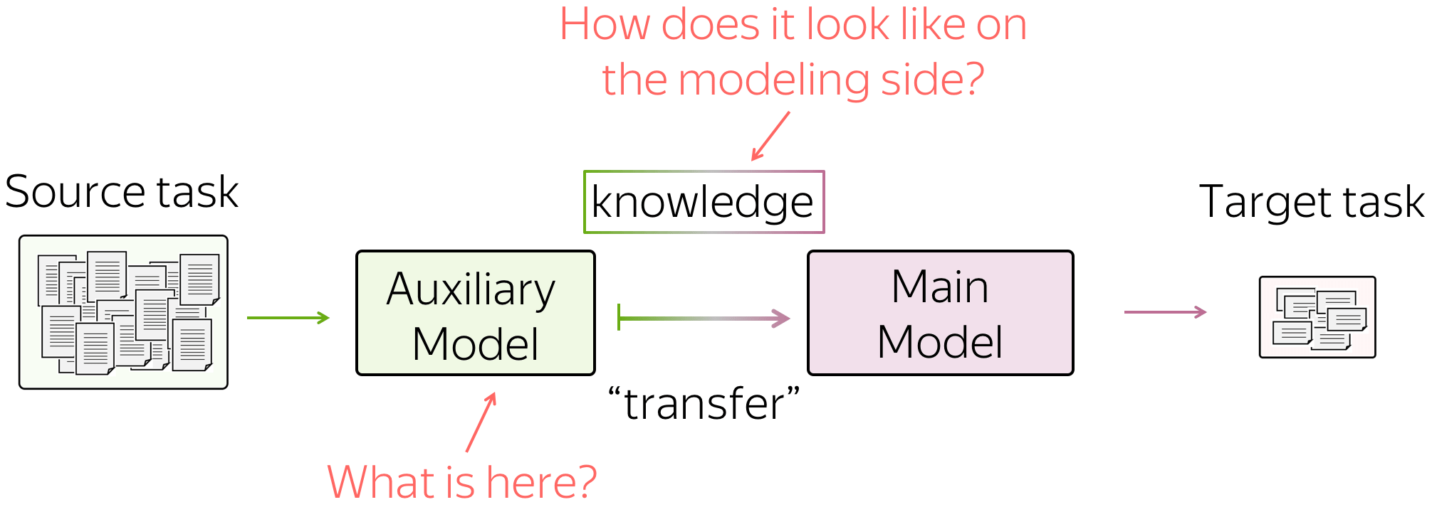
In this lecture, we are mostly interested in how the auxiliary models can look like and how the transfer itself looks on the modeling side.
The Simplest Transfer: Word Embeddings
When talking about Text Classification, we already discussed that using pretrained word embeddings can help a lot. Let's recap this part here.
Recap: Embeddings in Text Classification
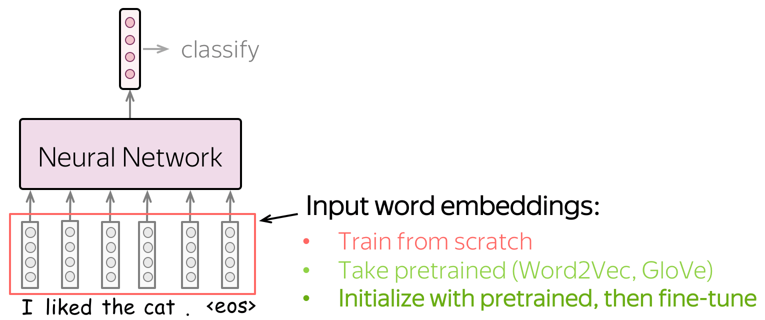
Input for a network is represented by word embeddings. You have three options on how to get these embeddings for your model:
- train from scratch as part of your model,
- take pretrained (Word2Vec, GloVe, etc) and fix them (use them as static vectors),
- initialize with pretrained embeddings and train them with the network ("fine-tune").
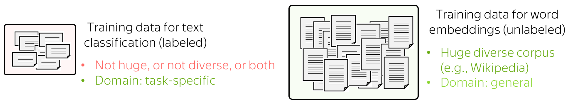
Let's think about these options by looking at the data a model can use. Training data for classification is labeled and task-specific, but labeled data is usually hard to get. Therefore, this corpus is likely to be not huge (at the very least), or not diverse, or both. On the contrary, training data for word embeddings is not labeled - plain texts are enough. Therefore, these datasets can be huge and diverse - a lot to learn from.
Now let us think about what a model will know depending on what we do with the embeddings. If the embeddings are trained from scratch, the model will "know" only the classification data - this may not be enough to learn relationships between words well. But if we use pretrained embeddings, they (and, therefore, the whole model) will know a huge corpus - they will learn a lot about the world. To adapt these embeddings to your task-specific data, you can fine-tune these embeddings by training them with the whole network - this can bring gains in performance (not huge though).
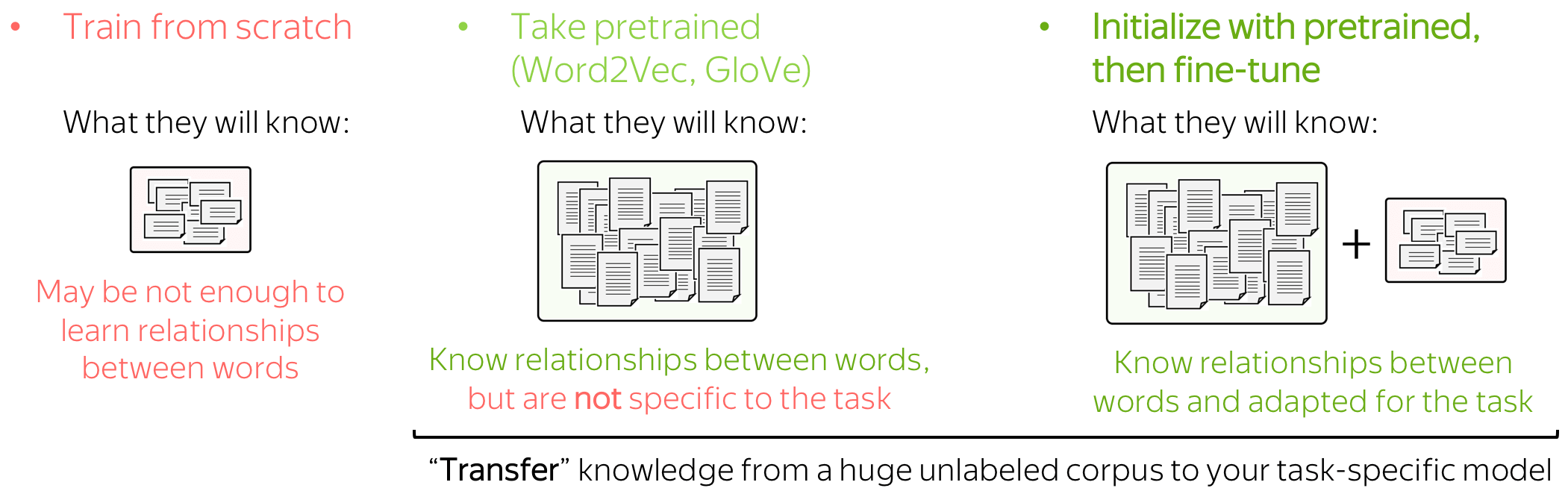
When we use pretrained embeddings, this is an example of transfer learning: through the embeddings, we "transfer" the knowledge of their training data to our task-specific model.
Transfer Through Word Embeddings
We just stated the main idea of using pretrained word embeddings in task-specific models:
Through the embeddings, we "transfer" the knowledge of their training data to our task-specific model.
In a model, this transfer is implemented via replacing randomly initialized embeddings with the pretrained ones (what is the same, copying weights from pretrained embeddings to your model).
Note that we do not change the model: it stays exactly the same. As we will see a bit later, this won't always be the case.
Pretrained Models
The idea of knowledge transfer we formulated for embeddings is general and stays the same when coming from word embeddings to pretrained models. I mean, literally the same: you can just replace "word embeddings" with your model's name!
Through _insert_your_model_, we "transfer" the knowledge of its training data to a task-specific model.
The Two Great Ideas
In this part, we are going to see 4 models: CoVe, ELMo, GPT, BERT. Note that now there are lots of variations of these models: ranging from very small modifications (e.g., training data and/or setting) to rather prominent ones (e.g., different training objectives). However, roughly speaking, the transition from word embeddings to the current state-of-the-art models can be explained with just two ideas.
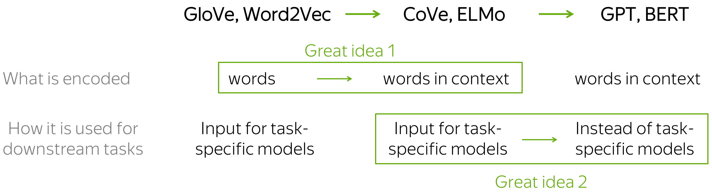
The two great ideas:
- what is encoded: from words to words-in-context
(the transition from Word2Vec/GloVe/etc. to Cove/ELMo); - usage for downstream tasks:
from replacing only word embeddings in task-specific models to replacing entire task-specific models
(the transition from Cove/ELMo to GPT/BERT).
Now, I will explain each of these ideas along with the corresponding models.
Great Idea 1: From Words to Words-in-Context
As we just saw, knowledge transfer through learned vector representations existed long before pretrained models: in the simplest case, through representations of words. What made transfer much more effective (and, therefore, popular) is a very simple idea:
Instead of representing individual words, we can learn to represent words along with the context they are used in.
Well, okay. But how do we do this?
Remember we trained neural language models? To train such a model you need the same kind of data that is used to train word embeddings: plain texts in natural language (e.g., Wikipedia texts, of anything you want). Note that for this you don't need any kind of labels!
Imagine now that we have some texts in natural language. We can use them to train word embeddings (Word2Vec, GloVe, etc.) or a neural language model. But by training a language model we get much more than by training word embeddings: language models process not just individual words, but sentences/paragraphs/etc. Inside a model, LMs too build vector representations for each word, but these vectors represent not just words, but words in context.
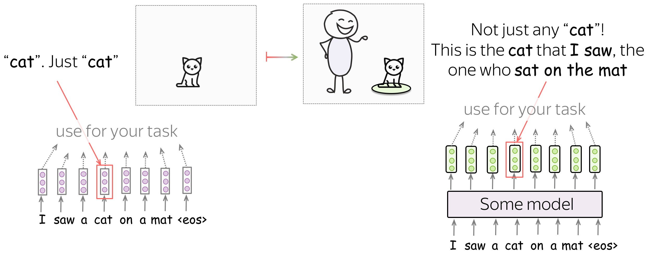
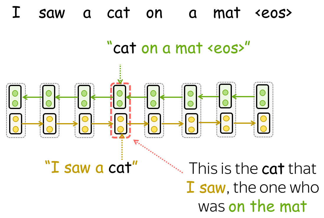
For example, let us look at the sentence I saw a cat on a mat and the word cat in it. If we use word embeddings, the vector for cat will contain information about the general notion of cat: this can be any kind of cat you can imagine. But if we take a vector for the cat from somewhere inside a language model, this won't be any cat anymore! Since LMs read the context, this vector representation for cat will know that this is the cat that I saw, the one who sat on the mat.
Transfer: Put Representations Instead of Word Embeddings
We are going to see the two models that first implemented the idea of encoding words with context: CoVe and ELMo. The way their representations are used for downstream tasks is almost the same as with word embeddings: usually, you just have to put representations instead of word embeddings (the place where previously you put e.g. GloVe). That's it!
Note that here you still have a task-specific model for each task, and these task-specific models can be quite different. What's changed is the way we encode words before feeding them to these task-specific models.
Lena: In the original papers, the authors propose some modifications for the task-specific models. These, however, are rather small, and roughly speaking can be ignored. What does matter is that instead of representing individual words, CoVe and ELMo represent words in context.
Now, all that's left is to specify
- this some model from the illustration,
- which representations to take from this model.
CoVe: Contextualized Word Vectors Learned in Translation
CoVe stands for "Context Vectors" and was introduced in the NeurIPS 2017 paper Learned in Translation: Contextualized Word Vectors. The authors first proposed to learn how to encode not only individual words but words along with their context.
Model Training: Neural Machine Translation (LSTMs and Attention)
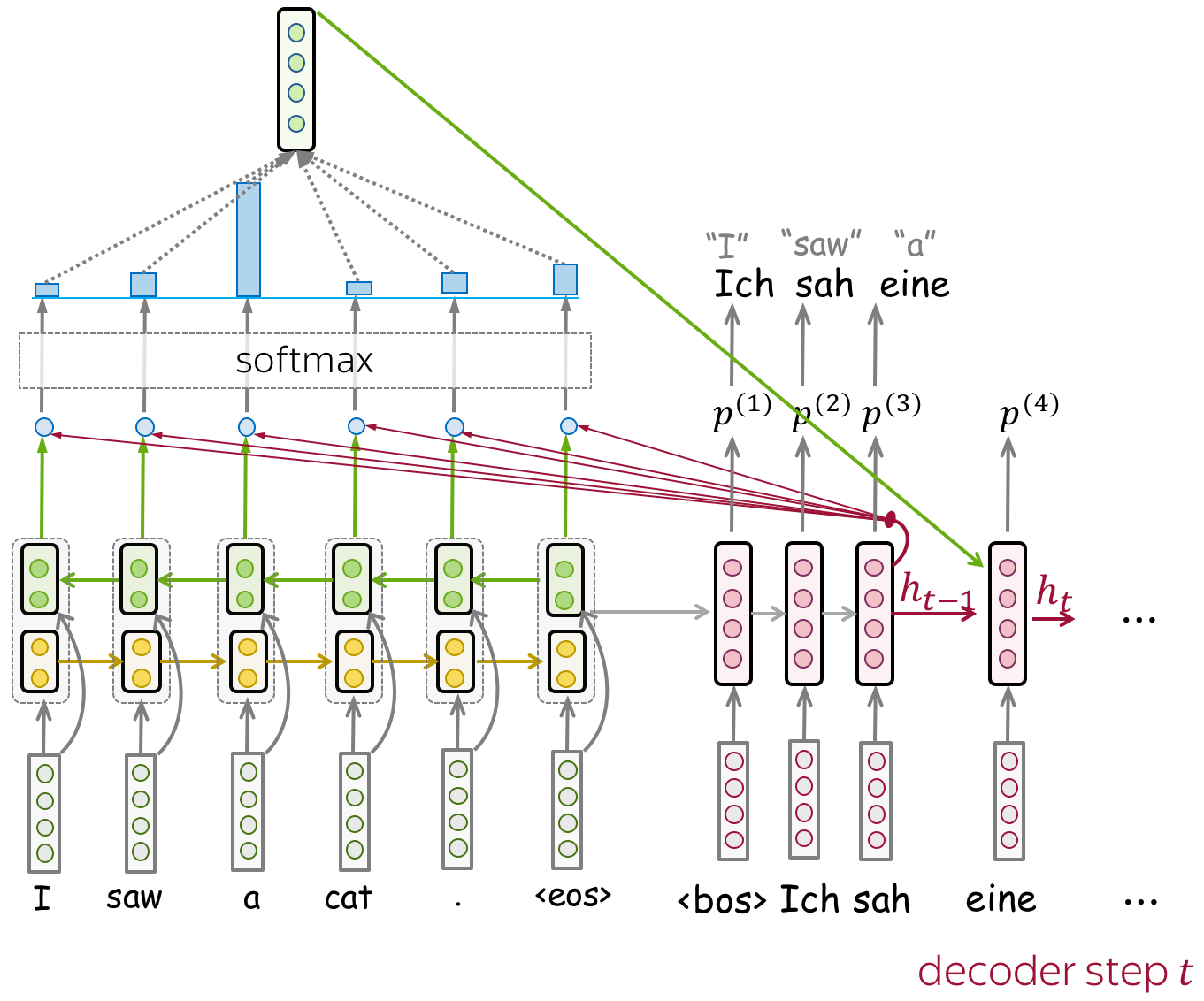
To encode words in the context of a sentence/paragraph, CoVe train an NMT system and use its encoder. The main hypothesis is that to translate a sentence, NMT encoders learn to "understand" the source sentence. Therefore, vector representations from the encoder contain information about a word's context.
Formally, the authors train an LSTM translation model with attention (e.g., Bahdanau model we saw in the previous lecture). Since in the end we want to use a trained encoder to process sentences in English (not because we care only about English, but because most of the datasets for downstream tasks are in English), the NMT system has to translate from English to some other language (e.g., German).
Bidirectional Encoder: Knows Both Left and Right Contexts
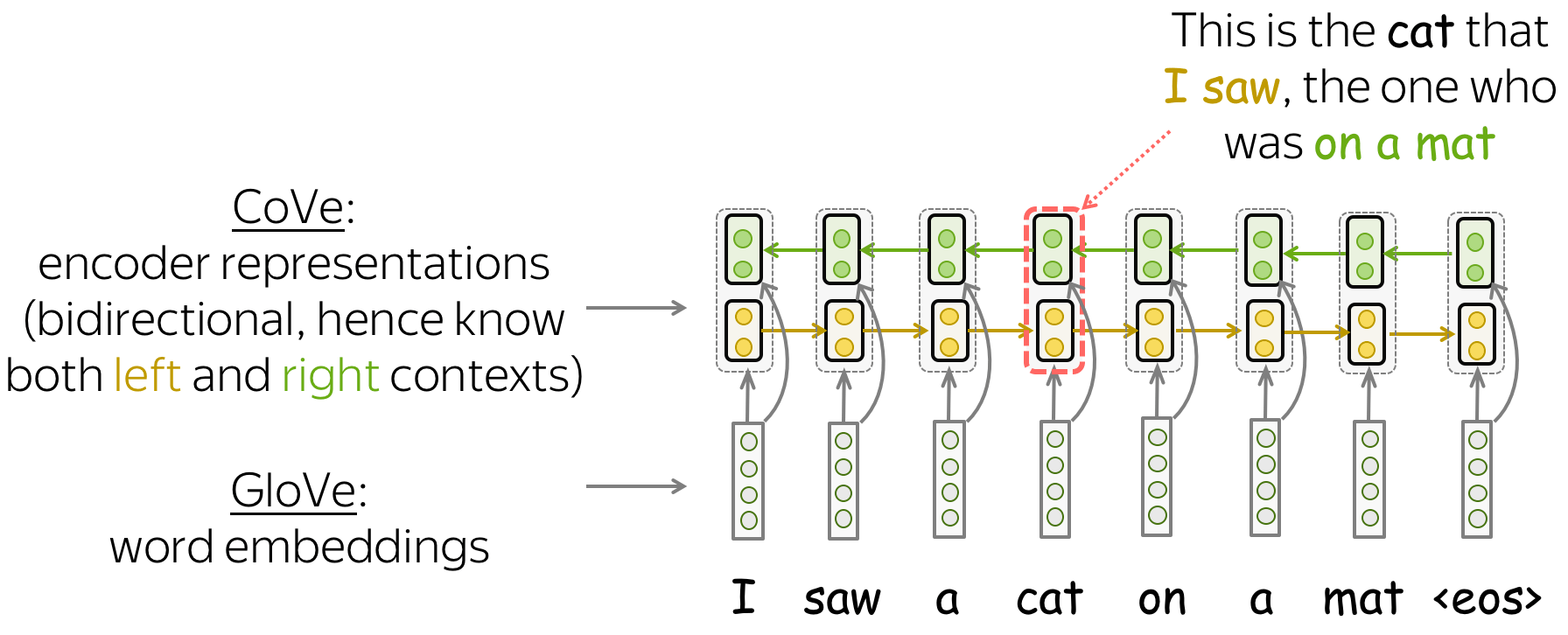
Note that in this NMT model, the encoder is bidirectional: it concatenates outputs of the forward and backward LSTMs. Therefore, encoder output contains information about both left and right contexts of a token.
Getting Representations: Concatenate GloVe and Cove Vectors
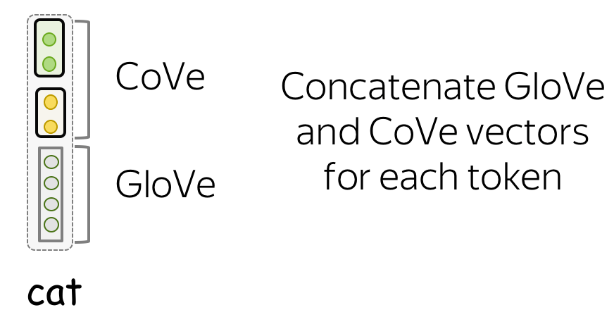
Once an NTM model is trained, we need only its encoder. For a given text, CoVe vectors are encoder outputs. For downstream tasks, the authors propose to use the concatenation of both Glove (which represent individual tokens) and CoVe (tokens encoded in context) vectors. The idea is that these vectors encode different kinds of information, and a combination of them can be useful.
Results: The Improvements are Prominent
Just by using CoVe vectors along with GloVe, the authors got prominent improvements on many downstream tasks: text classification, natural language inference and question answering.
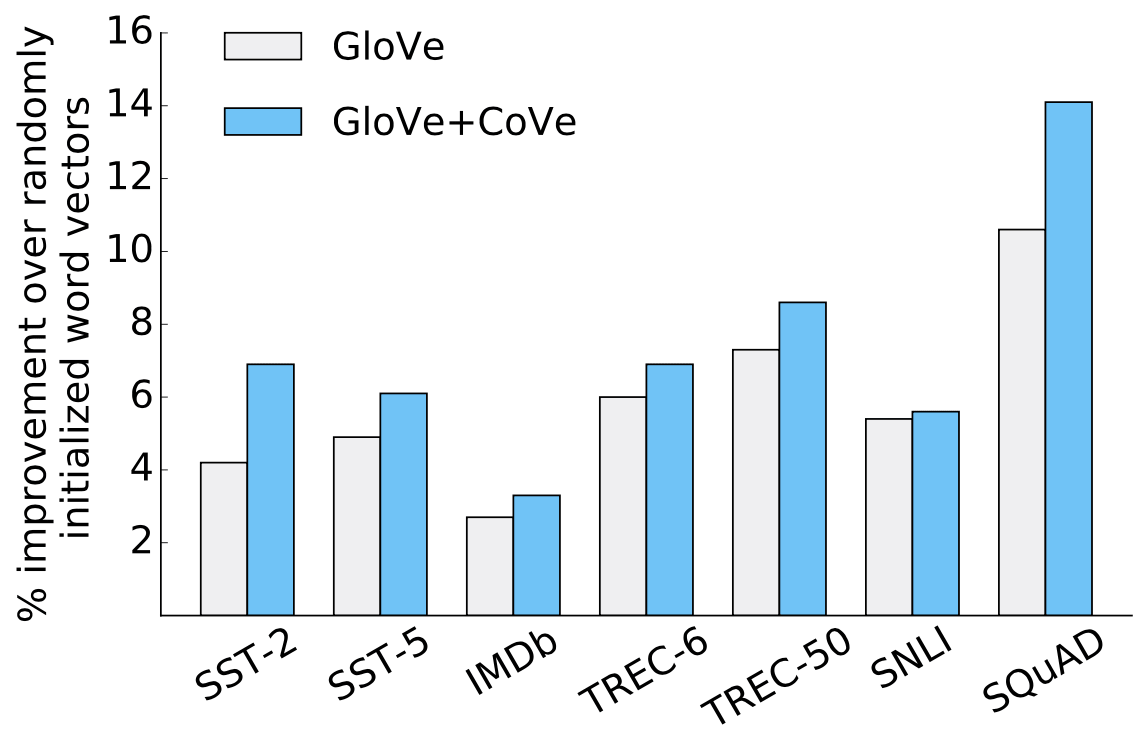
The figure is from the
the original CoVe paper.
ELMo: Embeddings from Language Models
The ELMo model was introduced in the paper Deep contextualized word representations. Differently from CoVe, ELMo uses representations not from NMT model, but from a language model. Just by replacing word embeddings (GloVe) with embeddings from LM they got a huge improvement for several tasks such as question answering, coreference resolution, sentiment analysis, named entity recognition, and others. And, by the way, the paper got the Best Paper Award at NAACL 2018!
Now let's look at ELMo in detail.
Model Training: Forward and Backward LSTM-LMs on top of char-CNN
The model is very simple and it consists of the two-layer LSTM language models: forward and backward. The two models are used so that each token could have both contexts: left and right.
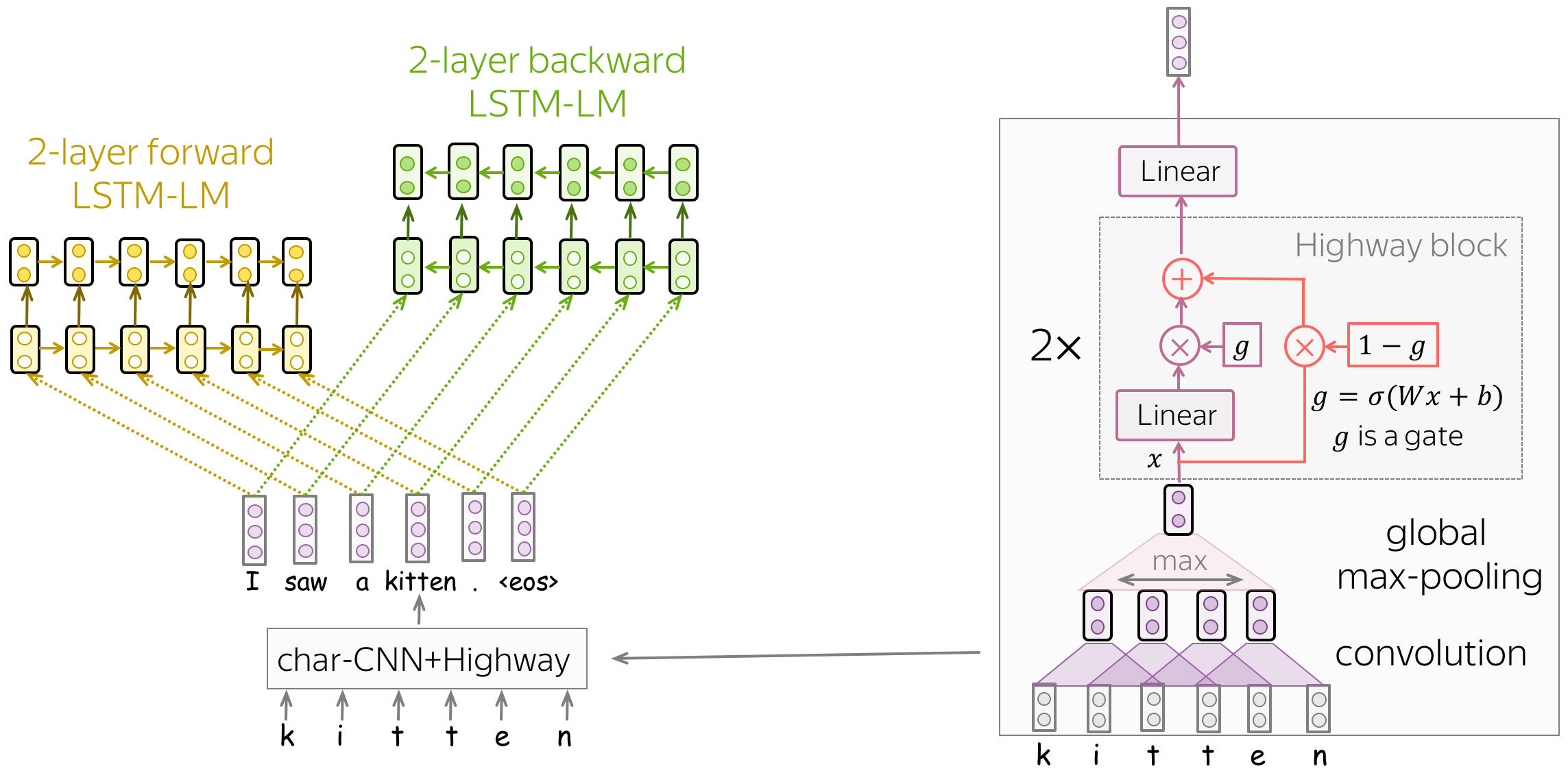
What is also interesting, is how the authors get initial word representations (which are then fed to the LSTMs). Let us recall that in the standard word embedding layer, for each word in the vocabulary we train a unique vector. In this case,
- word embeddings do not know the characters they consist of (e.g., they don't know that the words represent, represents, represented, and representation are close in writing)
- we can not represent out-of-vocabulary (OOV) words.
To address these problems, the authors represent words as outputs of a character-level network. As we see from the illustration, this CNN is very simple and consists of the components we already saw before: convolution, global pooling, highway connections, and linear layers. In this way, word representations know their characters by construction, and we can represent even those words we've never seen in training.
Getting Representations: Weight Representations from Different Layers
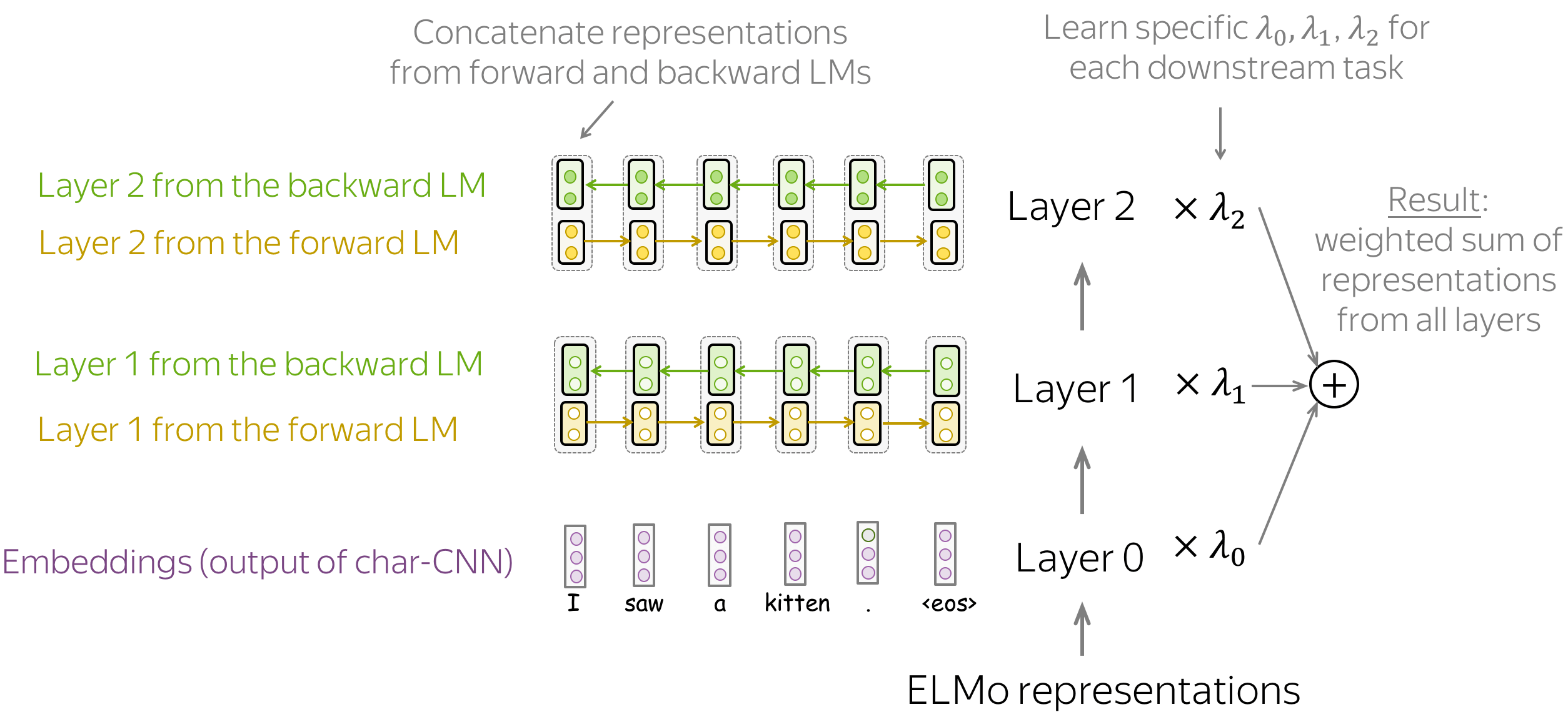
Once the model is trained, we can use it to get word representations. For this, for each word we combine representations from the corresponding layers from the forward and backward LSTMs. By concatenating these forward and backward vectors we construct a word representation that "knows" about both left and right contexts.
Overall, ELMo representations have three layers:
- layer 0 (embeddings) - output of the character-level CNN;
- layer 1 - concatenated representations from layer 1 of both forward and backward LSTMs;
- layer 2 - concatenated representations from layer 2 of both forward and backward LSTMs.
Layers contain different information → combine them
Each of these layers encodes different kinds of information: layer 0 - only word-level, layers 1 and 2 - words in context. Comparing between layers 1 and 2, layer 2 is likely to contain more high-level information: these representations come from the higher layers of the corresponding LMs.
Since different downstream tasks need different kinds of information, ELMo uses task-specific weights to combine representations from the three layers. These are scalars that are learned for each downstream task. The resulting vector, the weighted sum of representations from all layers, is used to represent a word.
Great Idea 2: Refuse From Task-Specific Models
The next two (classes of) models we are going to see are GPT and BERT which are very different from the previous approaches in a way they are used for downstream tasks:
CoVe/ELMo replace word embeddings, but GPT/BERT replace entire models.
Before: Specific model architecture for each downstream task
Note that ELMo/CoVe representations were mainly used to replace the embedding layer, and kept task-specific model architectures almost intact. This means e.g. that for coreference resolution, one had to use a specific model designed for this task, for part-of-speech tagging - some other model, for question answering - another, very peculiar model, etc. For each of these tasks, researchers specializing in it kept improving the task-specific model architectures.
After: Single model which can be fine-tuned for all tasks
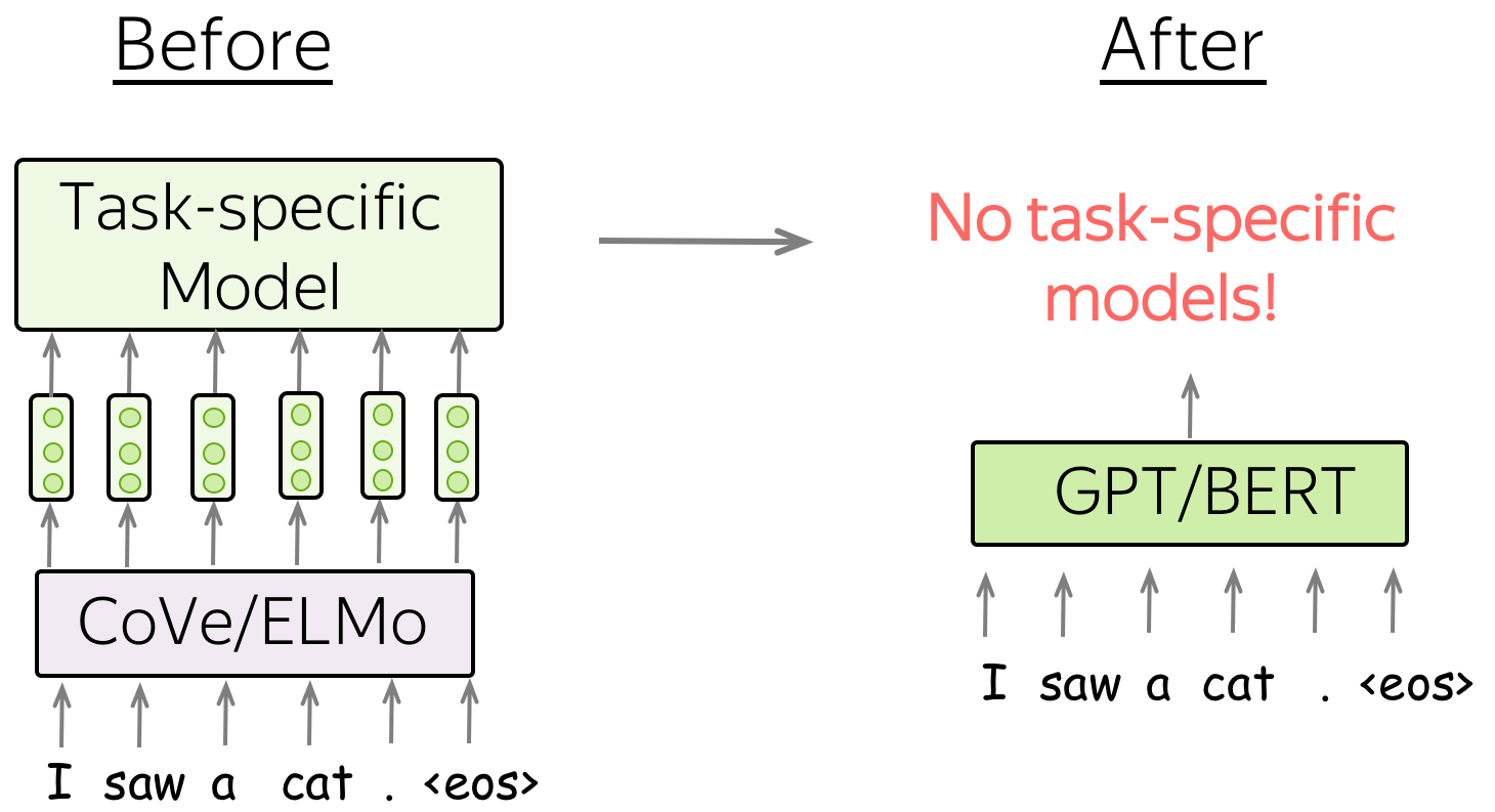
In contrast to previous models, GPT/BERT act not as a replacement for word embeddings, but as a replacement for task-specific models. In this new setting, a model is first pretrained using a huge amount of unlabeled data (plain texts). Then, this model is fine-tuned on each of the downstream tasks. What is important, now during fine-tuning you have to only use task-aware input transformations (i.e. feed the data in a certain way) instead of modifying model architecture.
GPT: Generative Pre-Training for Language Understanding
Pre-Training: Left-to-right Transformer Language Model
GPT is a Transformer-based left-to-right language model. The architecture is a 12-layer Transformer decoder (without decoder-encoder attention).
Formally, if \(y_1, \dots, y_n\) is a training token sequence, then at the timestep \(t\) a model predicts a probability distribution \(p^{(t)} = p(\ast|y_1, \dots, y_{t-1})\). The model is trained with the standard cross-entropy loss, and the loss for the whole sequence is
\[L_{xent}=-\sum\limits_{t=1}^n\log(p(y_t| y_{\mbox{<}t})).\]Lena: For more details on the left-to-right language modeling and/or Transformer model, see the Language Modeling and Seq2seq and Attention lectures.
Fine-Tuning: Using GPT for Downstream Tasks
The fine-tuning loss consists of the task-specific loss, as well as the language modeling loss:
\[L = L_{xent} + \lambda \cdot L_{task}.\]In the fine-tuning stage, the model architecture stays the same except for the final linear layer. What changes is the input format for each task: look at the illustration below.
![]()
The figure is from
the original GPT paper.
Single sentence classification
To classify individual sentences, just feed the data as in training and predict the label from the final representation of the last input token.
Examples of tasks:
- SST-2 - binary sentiment classification (the one we saw in the Text Classification lecture);
- CoLA (Corpus of Linguistic Acceptability) - say whether a sentence is linguistically acceptable.
Sentence pairs classification
To classify sentence pairs, feed the two fragments with a special token-separator (e.g. delim). Then, predict the label from the final representation of the last input token.
Examples of tasks:
- SNLI - entailment classification. Given a pair of sentences, say if the second is an entailment, contradiction or neutral);
- QQP (Quora Question Pairs) - given two questions say if they are semantically equivalent;
- STS-B - given two sentences return a similarity score from 1 to 5.
Question answering and commonsense reasoning
In these tasks, we are given a context document \(z\), a question \(q\), and a set of possible answers \(\{a_k\}\). Concatenate document and question, and after the delim token add a possible answer. For each of the possible answers, process the corresponding sequences independently with the GPT model; then normalize via a softmax layer to produce an output distribution over possible answers.
Examples of tasks:
- RACE - reading comprehension. Given a passage, a question and several answer options, pick the correct one.
- Story Cloze - story understanding and script learning. Given a four-sentence story and two possible endings, choose the correct ending to the story.
What is left: GPT-1-2-3 , Lots of Hype, and a Bit of Unicorns
So far, there are three GPT models:
- GPT-1: Improving Language Understanding by Generative Pre-Training
- GPT-2: Language Models are Unsupervised Multitask Learners
- GPT-3: Language Models are Few-Shot Learners
These models are different mostly in the amount of training data and the number of parameters (see, for example, this blog post. Note that these models are so big, that only huge companies can afford to train one. This gave rise to lots of discussions of concerns related to the use of such huge models (ethical, environmental, etc.). If you are interested in these, you can easily find lots of information on the internet.
But what you absolutely need to see, is the generated by GPT-2 story about unicorns in the Open AI blog post.
BERT: Bidirectional Encoder Representations from Transformers
BERT was introduced in the paper BERT: Pre-training of Deep Bidirectional Transformers for Language Understanding. If ELMo received the Best Paper Award at NAACL 2018, BERT did the same a year later, at NAACL 2019 :) Let's try to understand why.
BERT's model architecture is very simple and you already know how it works: it's just the Transformer's encoder. What is new, is the training objectives and the way BERT is used for downstream tasks.
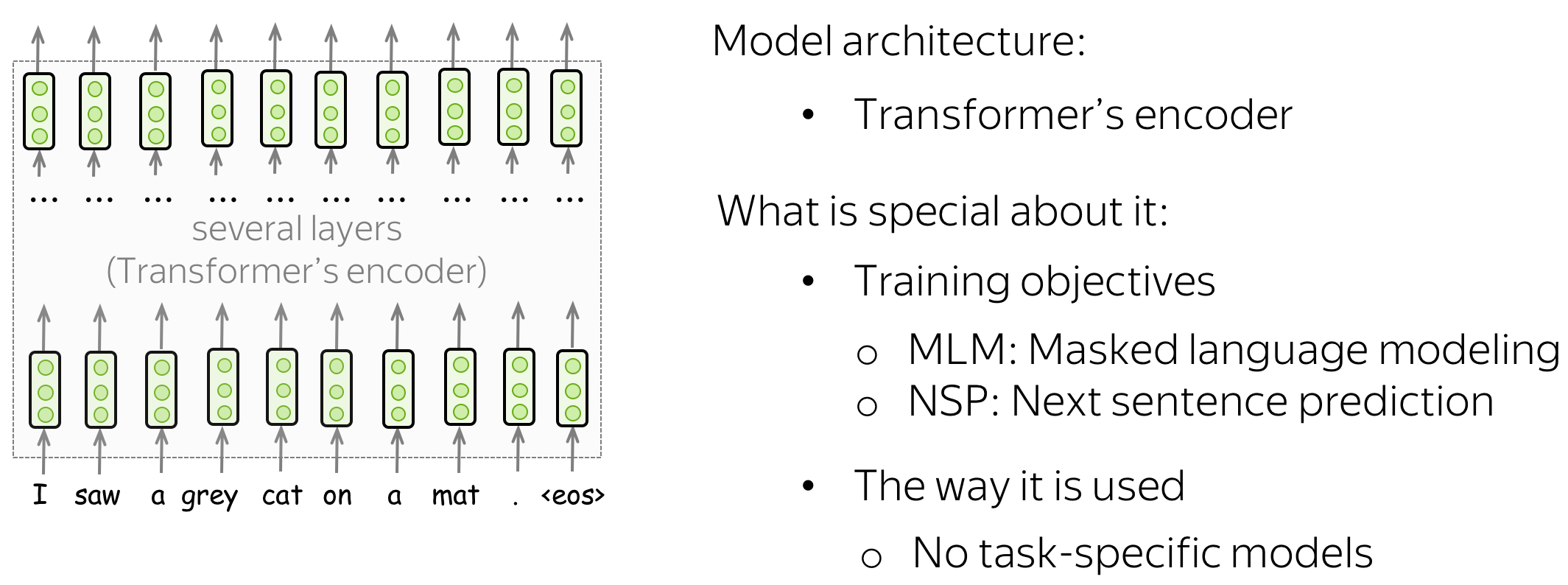
How can we train a (bidirectional) encoder using plain texts? We know only the left-to-right language modeling objective, but it is applicable only for decoders where each token can use only previous ones (and does not see the future). The BERT's authors came up with other training objectives for unlabeled data. Before we come to them, let's first look at what BERT gives as input to the Transformer's encoder.
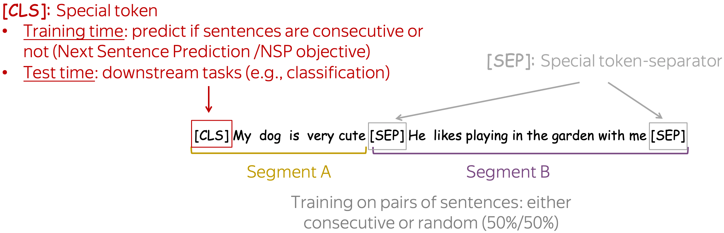
Training Input: Pairs of Sentences with Special Tokens
In training, BERT sees pairs of sentences separated with a special token-separator [SEP]. Another special token is [CLS]. In training, it is used for the NSP objective we'll see next. Once a model is trained, it is used for downstream tasks.
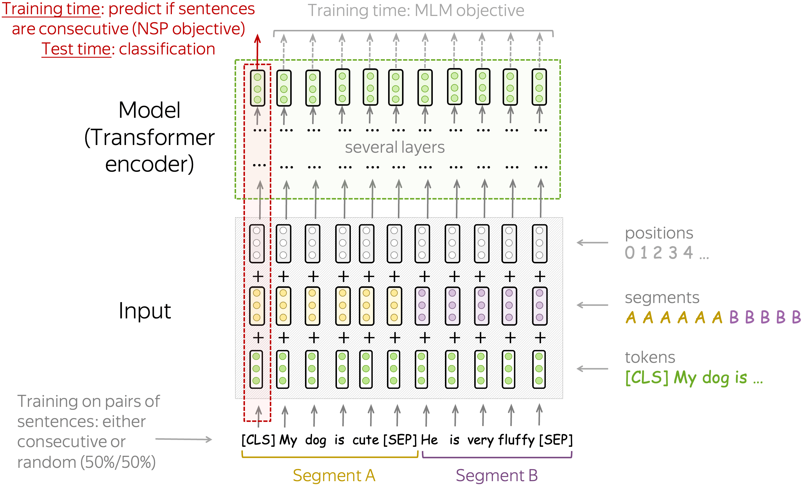
To let the model easily distinguish between these sentences, in addition to token and positional embeddings it uses segment embeddings. Overall, input for the model is sum of token, positional and segment embeddings. These representations are fed into transformer encoder, and the representations on top are used first for training, then for downstream applications.
Lena: Although, for downstream applications we can also use representations from the middle of the model. We will learn about this later.
Pre-Training Objectives: Next Sentence Prediction (NSP) Objective
The Next Sentence Prediction (NSP) objective is a binary classification task. From the final-layer representation of the special token [CLS], the model predicts whether the two sentences are consecutive sentences in some text or not. Note that in training, 50% of examples contain consecutive sentences extracted from training texts and another 50% - a random pair of sentences. Look at a couple of examples from the original paper.
Input: [CLS] the man went to [MASK] store [SEP] he bought a gallon [MASK] milk [SEP]
Label: isNext
Input: [CLS] the man went to [MASK] store [SEP] penguin [MASK] are flight ##less birds [SEP]
Label: notNext
This task teaches the model to understand the relationships between sentences. As we'll see later, this will enable to use BERT for complicated tasks requiring some kind of reasoning.
Pre-Training Objectives: Masked Language Modeling (MLM) Objective
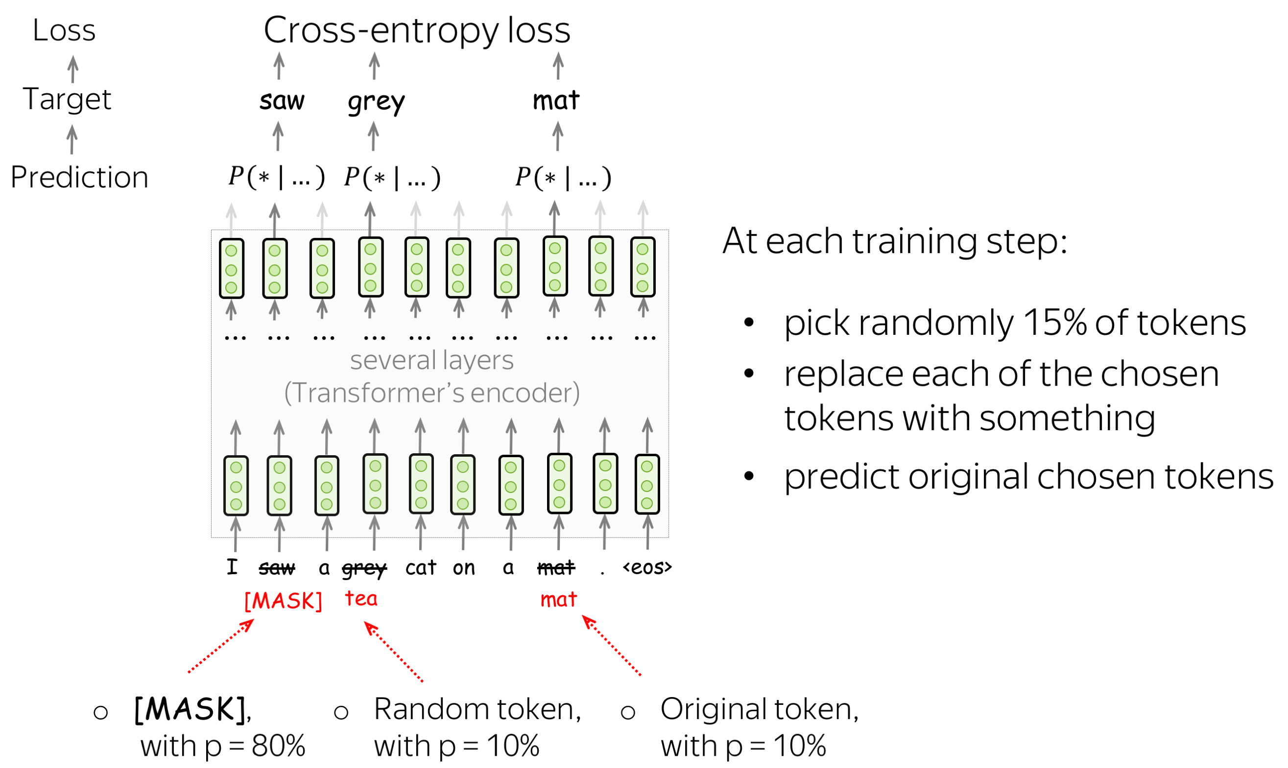
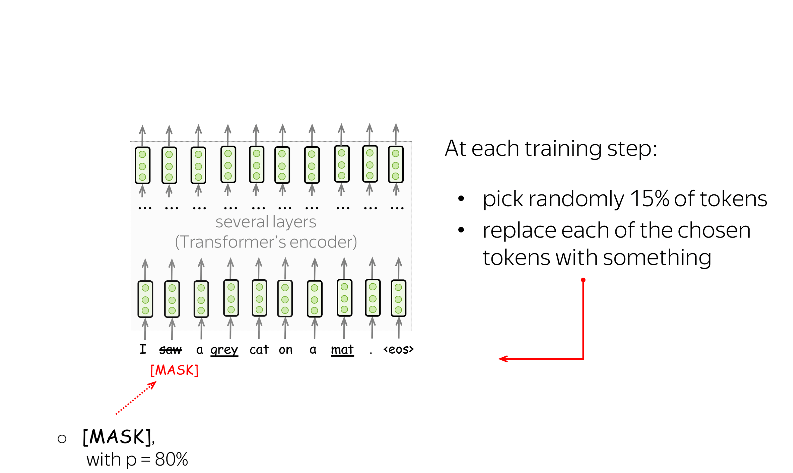
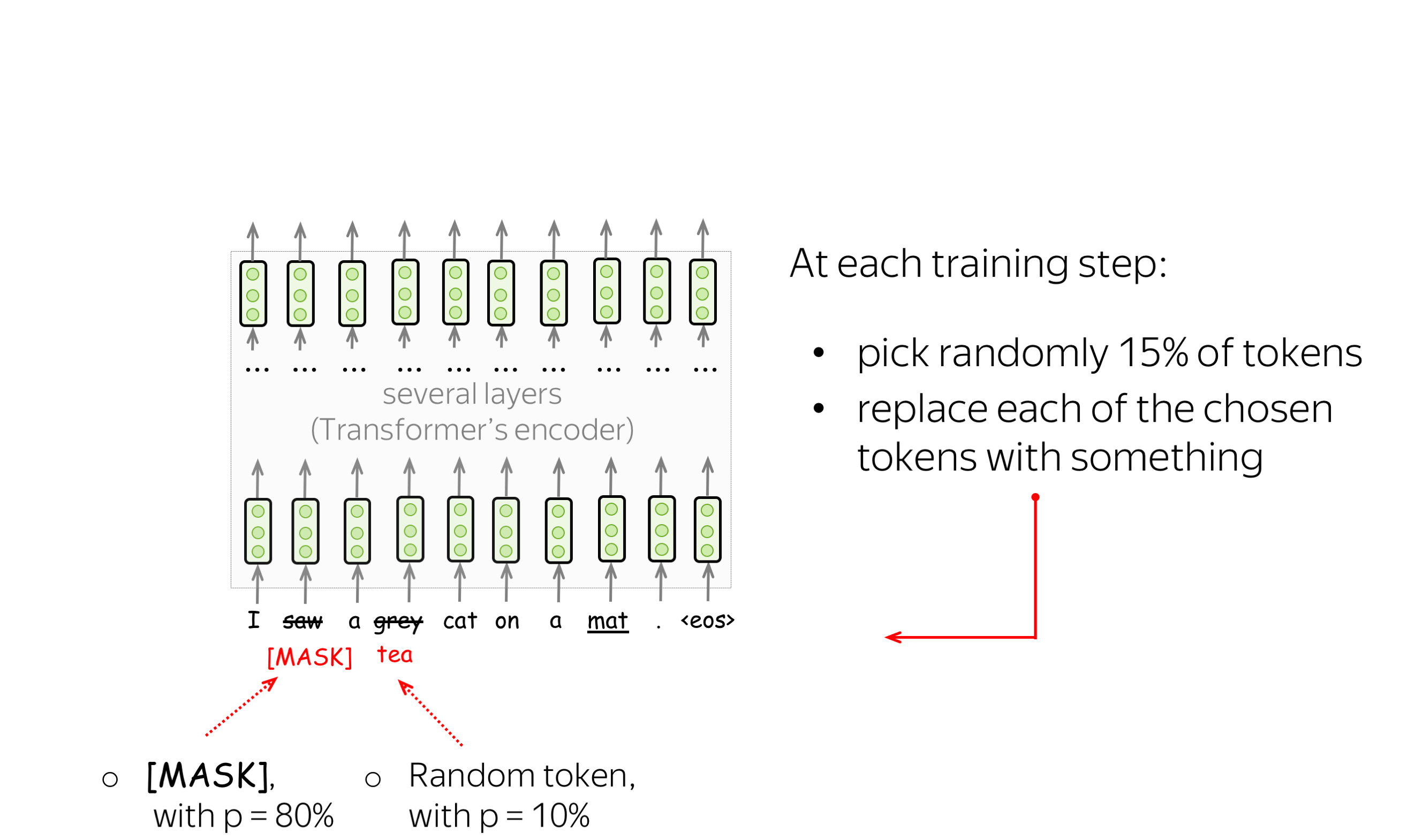
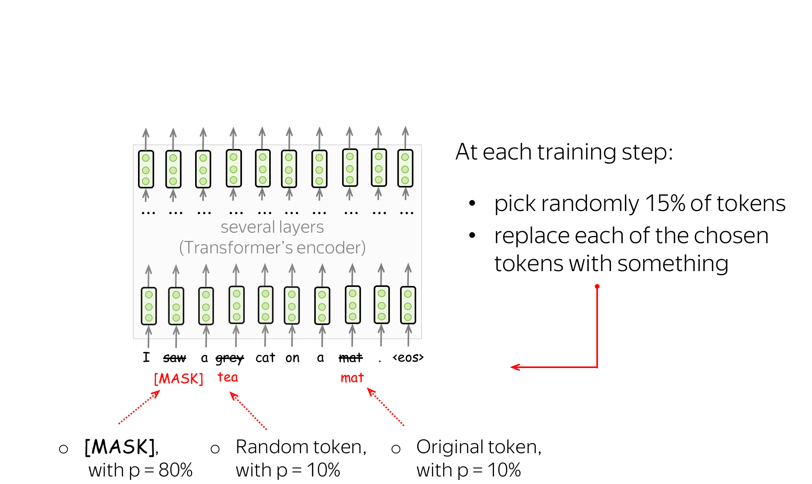
BERT has two training objectives, and the most important of them is the Masked Language Modeling (MLM) objective. is With the MLM objective, at step the following happens:
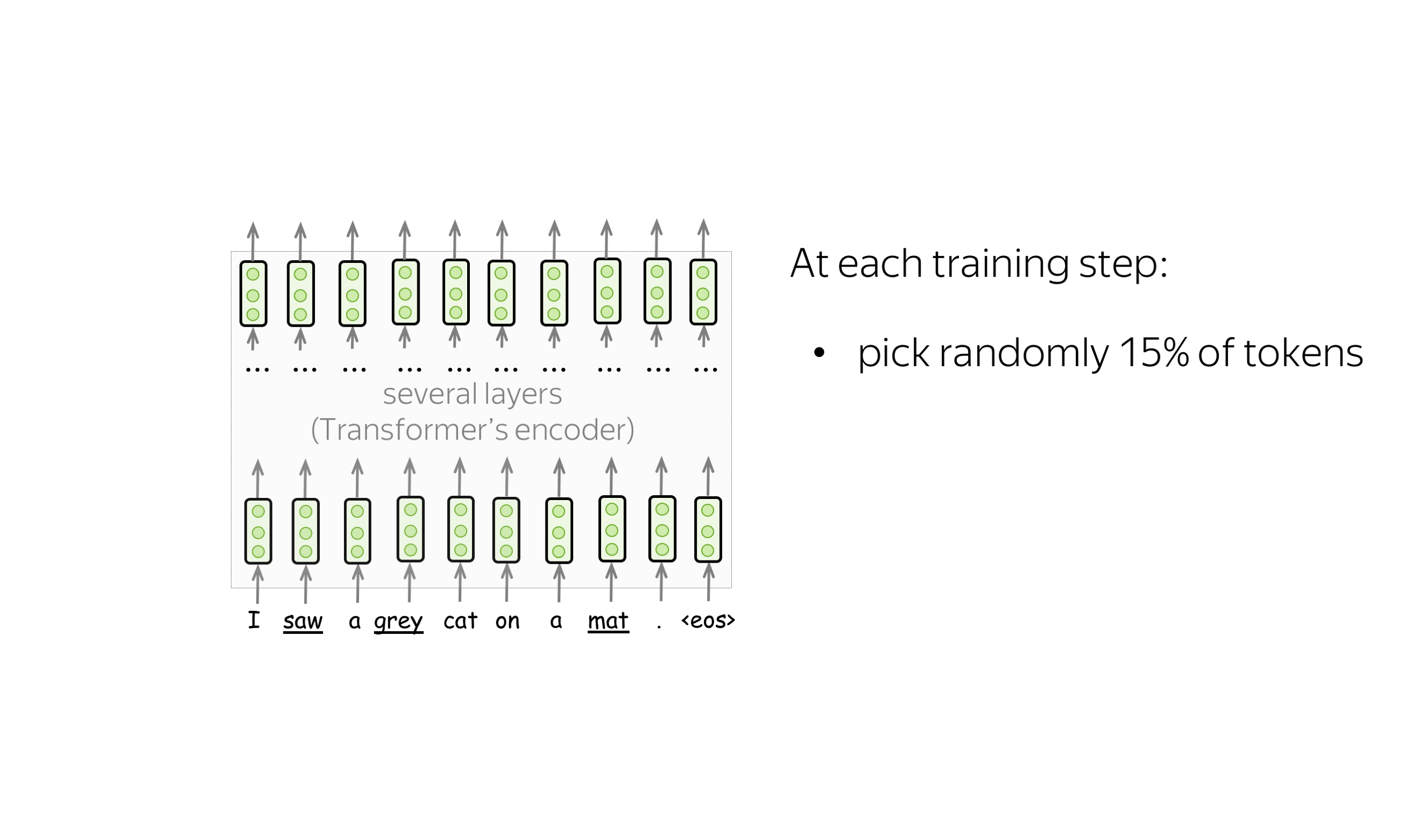
- select some tokens
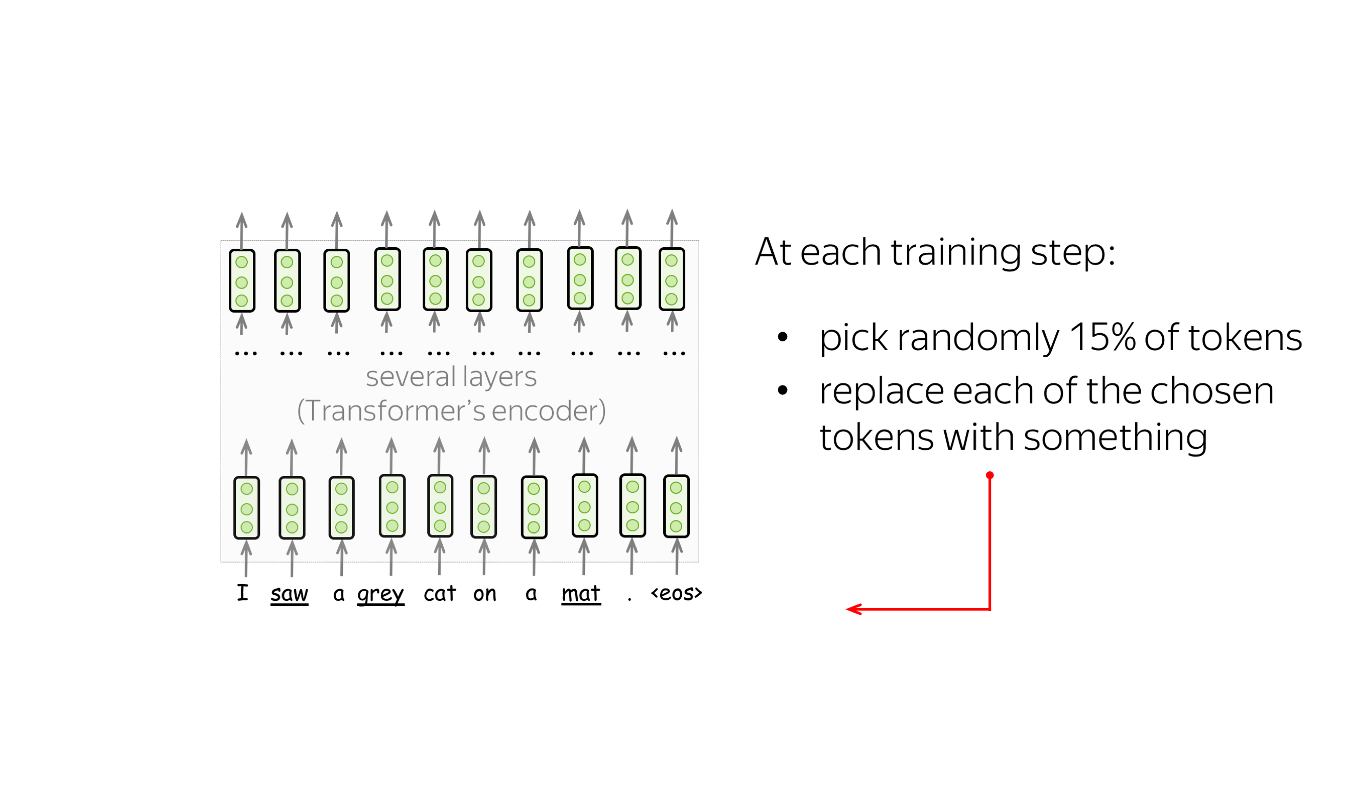
(each token is selected with the probability of 15%) - replace these selected tokens
(with the special token [MASK] - with p=80%, with a random token - with p=10%, with the original token (remain unchanged) - with p=10%) - predict original tokens (compute loss).
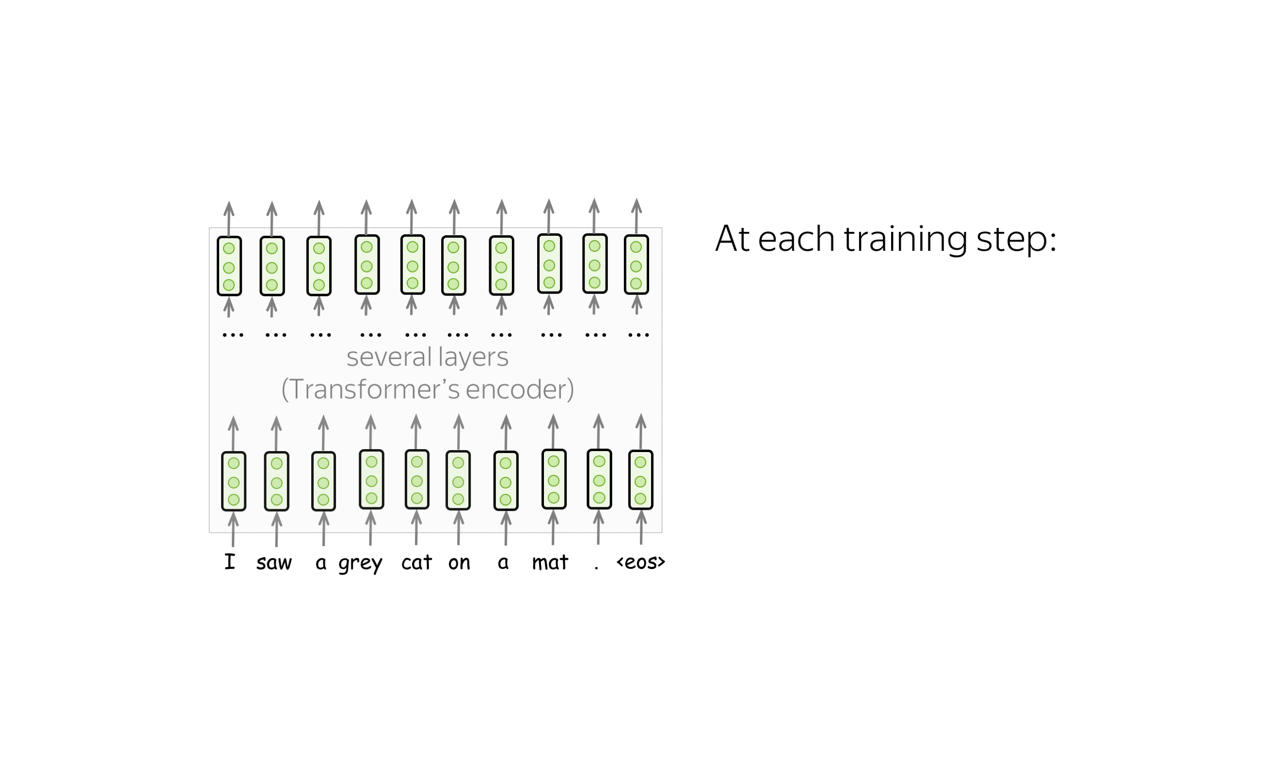
The illustration below shows an example of a training step for one sentence. You can go over the slides to see the whole process.
MLM is still language modeling: the goal is to predict some tokens in a sentence/text based on some part of this text. To make it more clear, let us compare MLM with the standard left-to-right language modeling objective.
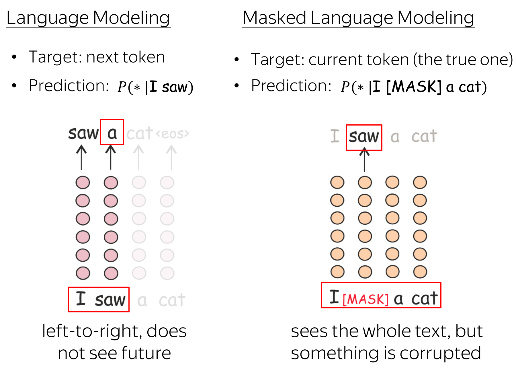
At each step, the standard left-to-right LMs predict the next token based on the previous ones. This means that final representations, the ones from the final layer that are used for prediction, encode only previous context, i.e. they do not see the future.
Differently, MLMs see the whole text at once, but some tokens are corrupted: that's why BERT is bidirectional. Note that to let ELMo know both left and right contexts, the authors had to train two different unidirectional LMs and then concatenate representations of both of them. In BERT, we don't need to do that: one model is enough.
Fine-Tuning: Using BERT for Downstream Tasks
Now let's look at how to apply BERT for different tasks. For now, we will only at the simple setting: when the pretrained model is fine-tuned on each of the downstream tasks. Later, we'll see other ways to adapt a model for different applications (e.g., in the Adapters section).
In this part, I'll mention only some of the tasks. For more details on the popular evaluation datasets, take a look at the GLUE benchmark website.
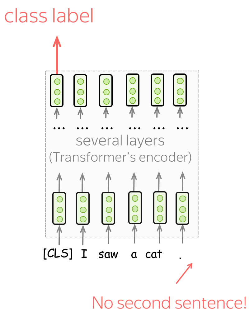
Single sentence classification
To classify individual sentences, feed the data as shown on the illustration and predict the label from the final representation of the [CLS] token.
Examples of tasks:
- SST-2 - binary sentiment classification (the one we saw in the Text Classification lecture);
- CoLA (Corpus of Linguistic Acceptability) - say whether a sentence is linguistically acceptable.
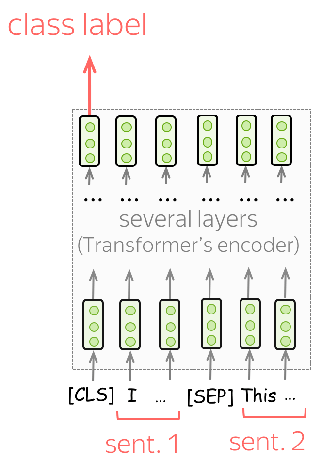
Sentence Pair Classification
To classify pairs of sentences, feed the data as you did in training. Similar to the single sentence classification, predict the label from the final representation of the [CLS] token.
Examples of tasks:
- SNLI - entailment classification. Given a pair of sentences, say if the second is an entailment, contradiction, or neutral);
- QQP (Quora Question Pairs) - given two questions, say if they are semantically equivalent;
- STS-B - given two sentences, return a similarity score from 1 to 5.
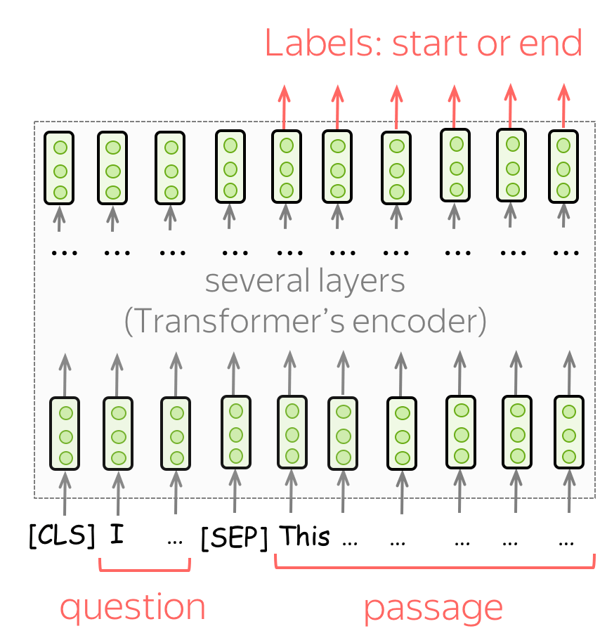
Question Answering
For QA, the BERT authors used only one dataset, SQuAD v1.1. In this task, you are given a text passage and a question. The answer to this question is always a part of the passage, and the task is to find the correct segment of the passage.
To use BERT for this task, feed a question and a passage as shown in the illustration. Then, for each token in the passage use final BERT representations to predict whether this token is the start or the end of the correct segment.
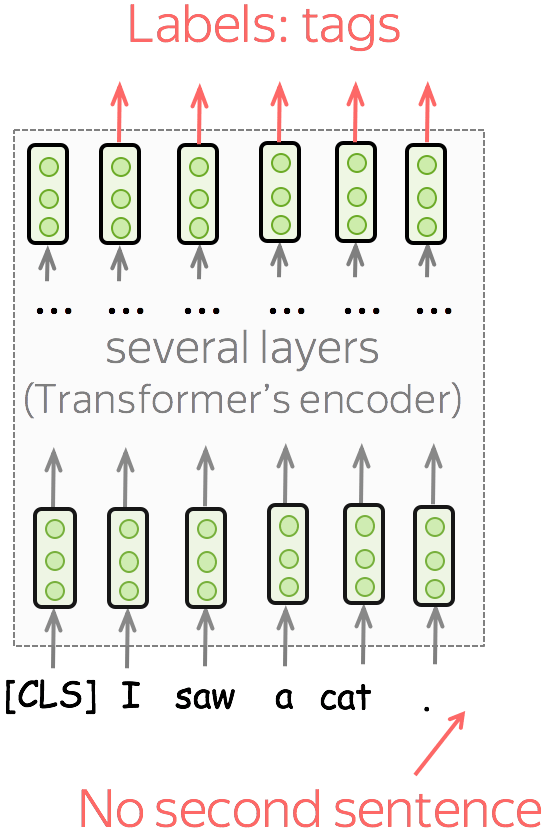
Single sentence tagging
In tagging tasks, you have to predict tags for each token. For example, in Named Entity Recognition (NER), you have to predict if a word is a named entity and its type (e.g., location, person, etc).
(A Bit of) Adapters: Parameter-Efficient Transfer
So far, we considered only the standard way of transferring knowledge from pretrained models (e.g. BERT) to downstream tasks: fine-tuning. "Fine-tuning" means that you take a pretrained model and train in for the task you are interested in (e.g., sentiment classification) with a rather small learning rate. This means that firstly, you update the whole (large) model, and secondly, for each task, you need to fine-tune a separate copy of your pretrained model. In the end, for several downstream tasks you end up with a lot of large models - this is highly inefficient!
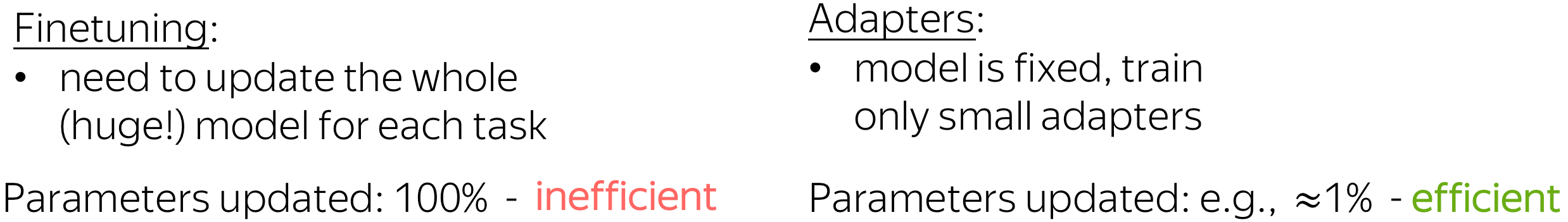
As an alternative, the ICML 2019 paper Parameter-Efficient Transfer Learning for NLP proposed transfer with adapter modules. In this setting, the parameters of the original model are fixed, and one has to train only a few trainable parameters per task: these new task-specific parameters are called adaptors. With adapter modules, transfer becomes very efficient: the largest part, the pretrained model, is shared between all downstream tasks.
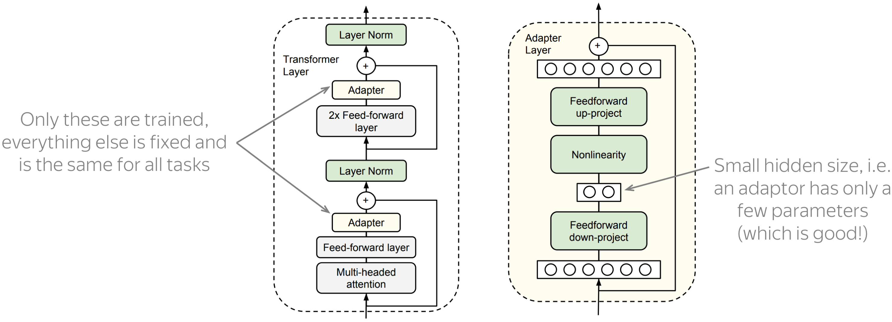
The figure is from the paper
Parameter-Efficient Transfer Learning for NLP.
An example of an adapter module and a transformer layer with adapters is shown in the figure. As you can see, an adapter module is very simple: it's just a two-layer feed-forward network with a nonlinearity. What is important, the hidden dimensionality of this network is small, which means that the total number of parameters in the adapter is also small. This is what makes adaptors very efficient.
Other Adapters and Some Resources
Now, there are many different modifications of adaptors for lots of tasks and models. For example, the AdapterHub repository contains pre-trained adapter modules. Since this was a system demo at EMNLP 2020, it can be a good starting point if you want to find links to the latest adapter versions (Lena: At least, at the moment I'm writing this: beginning of December 2020, i.e. only a couple of weeks after EMNLP 2020).
(A Note on) Benchmarks
The most popular benchmark is GLUE and its version SuperGLUE. The GLUE benchmark website contains dataset descriptions, leaderboard, etc.
Analysis and Interpretability
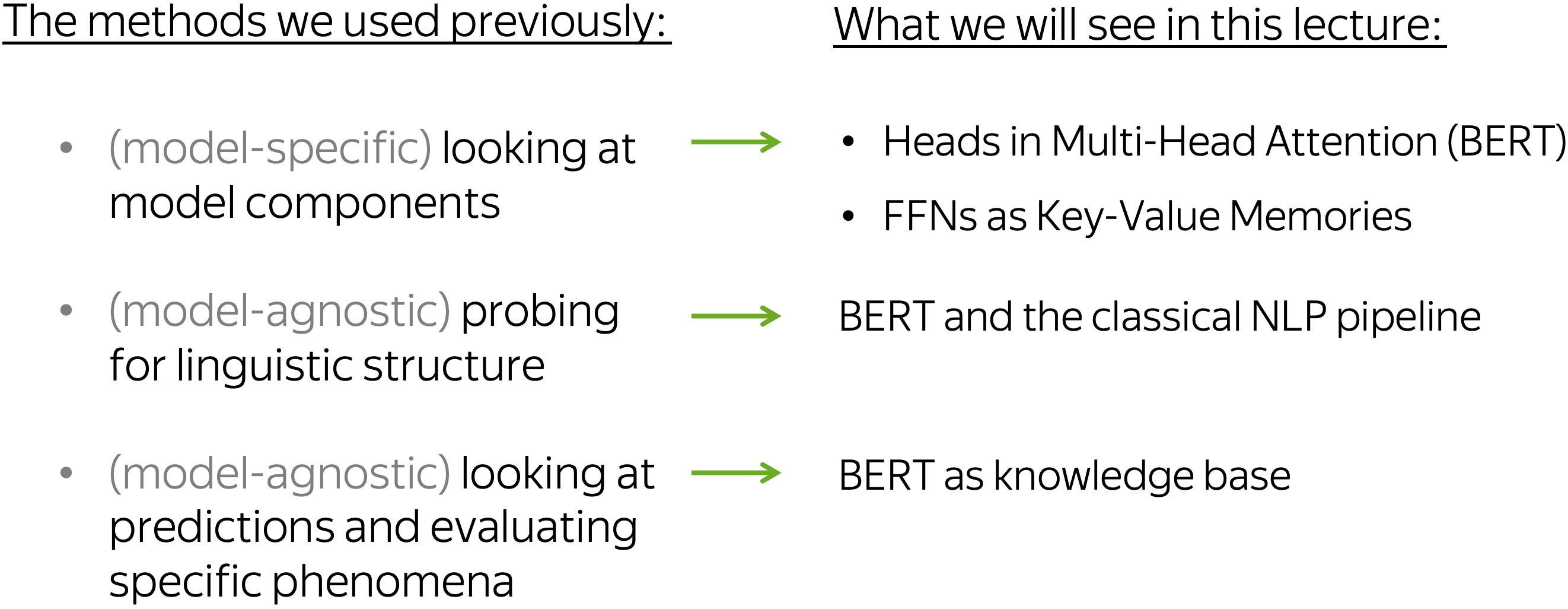
First, let us recap the analysis methods we already used in the previous lectures: looking at model components (e.g. neurons in CNNs/LSTMs and attention heads in Transformer), probing for linguistic structure (e.g., whether NMT representations encode information about morphology), and evaluating specific phenomena by looking at a model's predictions (e.g., evaluating subject-verb agreement in language models). Today, we will see what happens when the same methods are applied to BERT.
Model Components: BERT's Attention Heads
In the previous lectures, we looked at CNN filters in Text Classification, LSTM neurons in Language Models and attention heads in NMT Transformer. Now, let's look at what researchers found in the attention patterns of BERT's heads!
Simple patterns: Positional Heads, Attention to [SEP] and Period
Remember the positional self-attention heads we saw in the machine translation Transformer? Turns out, BERT also has such heads. The paper What Does BERT Look At? An Analysis of BERT’s Attention shows that some of the BERT's heads have simple patterns: not only positional (when all tokens attend to the previous or next token) but also heads putting all their attention mass to some tokens, e.g. the special token [SEP] of the period.
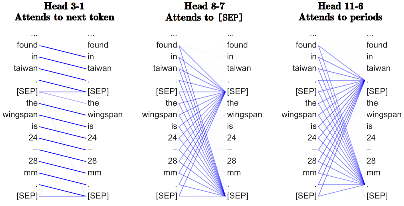
The examples are from the paper
What Does BERT Look At? An Analysis of BERT’s Attention.
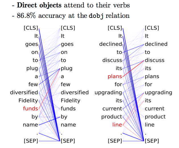
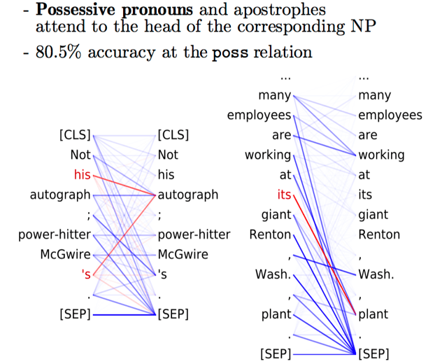
Examples of syntactic heads from the paper What Does BERT Look At? An Analysis of BERT’s Attention
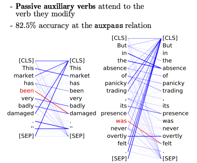
Examples of syntactic heads from the paper What Does BERT Look At? An Analysis of BERT’s Attention
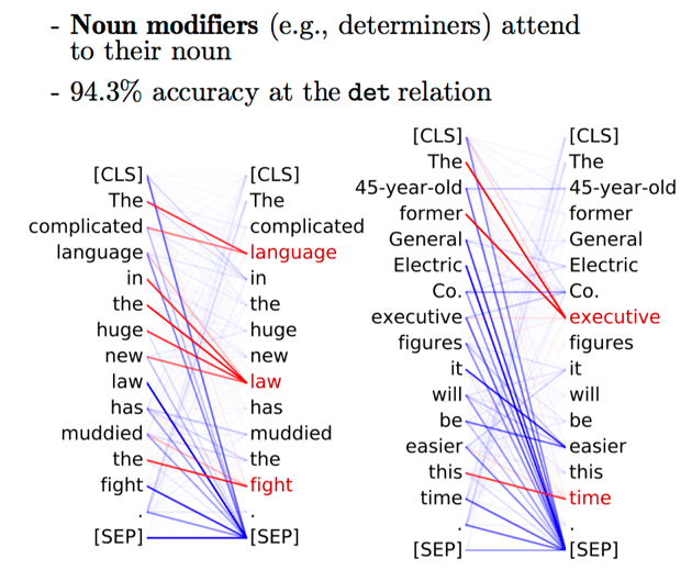
Examples of syntactic heads from the paper What Does BERT Look At? An Analysis of BERT’s Attention
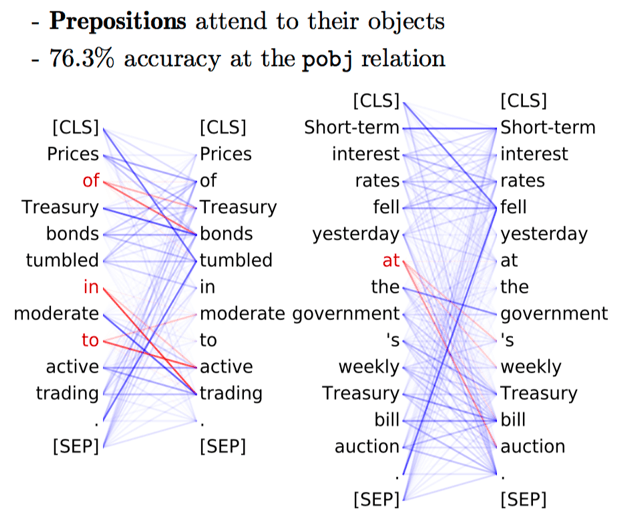
Examples of syntactic heads from the paper What Does BERT Look At? An Analysis of BERT’s Attention
Examples of syntactic heads from the paper What Does BERT Look At? An Analysis of BERT’s Attention
Syntactic Heads
Similar to syntactic self-attention heads found for NMT Transformer, there were also found several BERT heads that specialize in tracking certain syntactic functions. Look at the illustration.
Note that there are also some other works looking at attention functions in BERT. For example, Do Attention Heads in BERT Track Syntactic Dependencies? confirm that some BERT heads are indeed syntactic, while some other works fail to find heads that do this confidently. As always, you need to be very careful :)
Model Components: FFNs as Key-Value Memories
Transformer and the Residual Stream
As we learned in the previous lecture, in the Transformer (either encoder or decoder) a token representation evolves from the input token embedding to the final layer prediction. Via residual connections, attention and feed-forward blocks update the original representation by adding new information. This sequence of evolving representations for the same token is called the residual stream.
Note that while attention layers allow exchanging information across tokens, FFNs operate within the same residual stream. Now, let us look at this layer more closely.
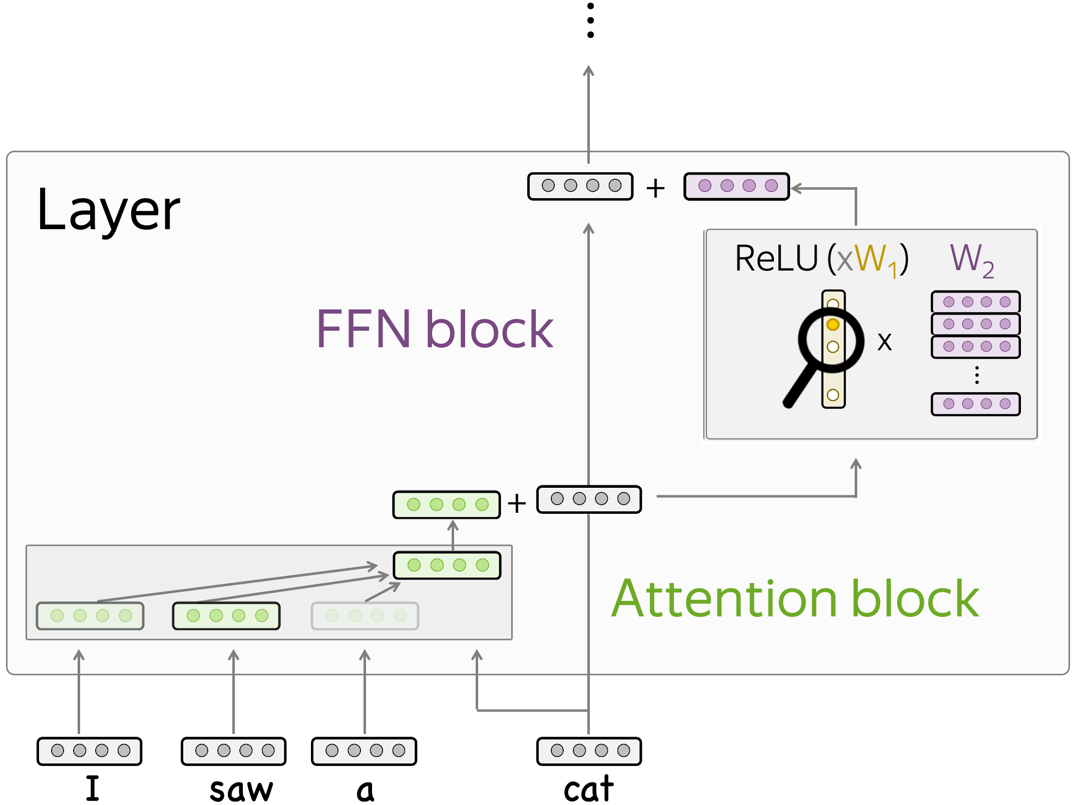
The Key-Value View of FFNs
In this paper, the authors propose to view feed-forward layers in transformer-based language models as key-value memories. In this view, the columns of the first FFN layer encode textual concepts and the rows of the second FFN layer encode distributions over vocabulary.
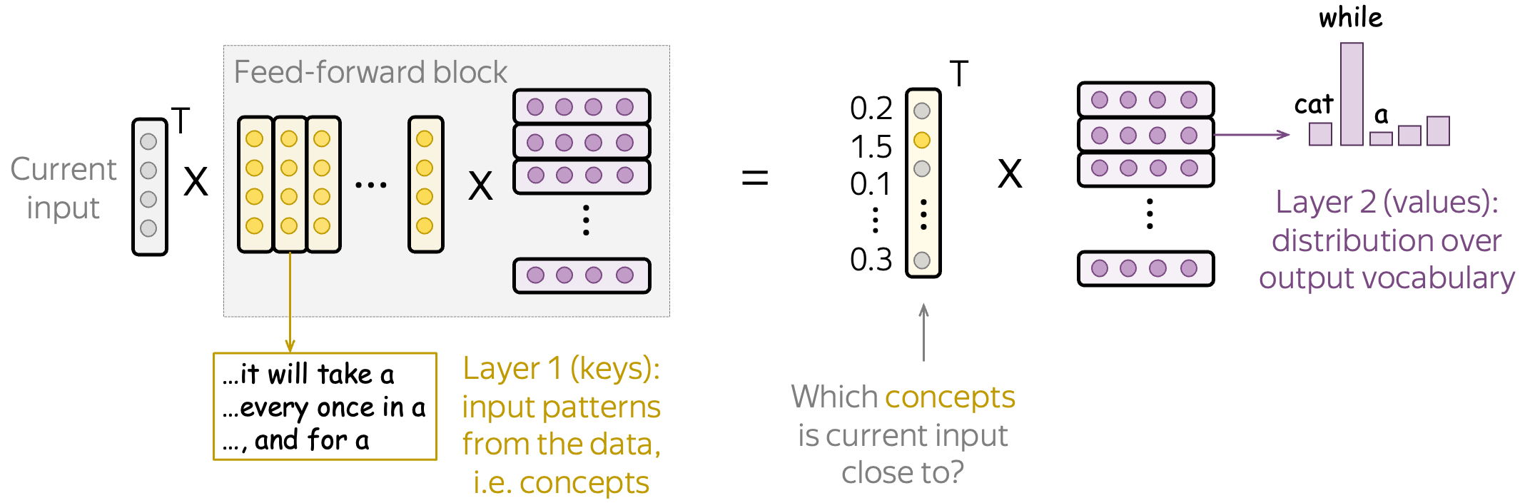
When our input vector goes into the FFN block, it first matches some of the concepts encoded in the first layer and receives the weights - in our illustration, this is shown in yellow. Then, these weights trigger the corresponding rows or the second FFN layer. These rows (multiplied by the weights) will update the output token distribution encoded in the residual stream.
Probing: BERT Rediscovers the Classical NLP Pipeline
Now there are plenty of papers applying probing to BERT. In this part, let's look at the ACL 2020 short paper BERT Rediscovers the Classical NLP Pipeline.
How: Probing with a Bit of Creativity
In the previous lecture we learned about standard probing for linguistic structure:
- feed the data to your pretrained model,
- get vector representations from some layer,
- train a probing classifier to predict linguistic labels from representations,
- use its accuracy as a measure of how well representations encode these labels.
Of course, this can be done for BERT, too. But BERT has lots of layers (e.g., 18 or 24) and to understand which layers better encode a certain task we would have to train 18 (or 24) probing classifiers for each task - this is lots of work!
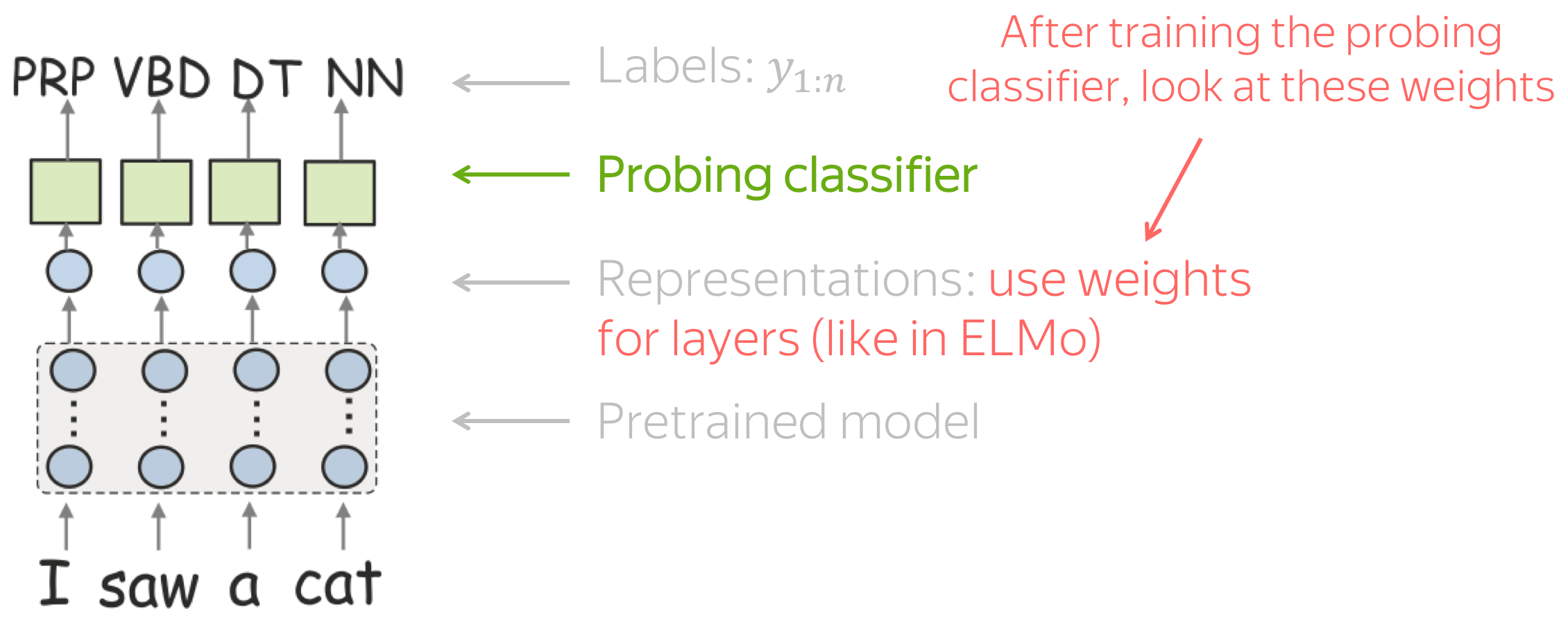
Luckily, the authors came up with a way to evaluate all layers at once. Instead of picking representations from each layer separately, to train a probing classifier they weight representations from all layers and learn the weights with a probing classifier (just like in ELMo!). Once the probing classifier is trained, the weights can serve as a measure of a layer's importance for a certain task.
What: Edge Probing Tasks
The authors experiment with a set of edge probing tasks. These are test sets for several linguistic tasks. Look at some examples below.
•part of speech
I want to find more , [something] bigger or deeper .
→ NN (Noun)
•constituents
I want to find more , [something bigger or deeper] . → NP (Noun Phrase)
•dependencies
[I]\(_1\) am not [sure]\(_2\) how reliable it is , though . → nsubj (nominal subject)
•entities
The most fascinating is the maze known as [Wind Cave] . → LOC (location)
•semantic role labeling
I want to [find]\(_1\) [something bigger or deeper]\(_2\) . → Arg1 (Agent)
•coreference
So [the followers]\(_1\)
wanted to say anything about what [they]\(_2\)
saw . → True
Results: BERT Follows the Classical NLP Pipeline
The figure with the results is from the paper
BERT Rediscovers the Classical NLP Pipeline.
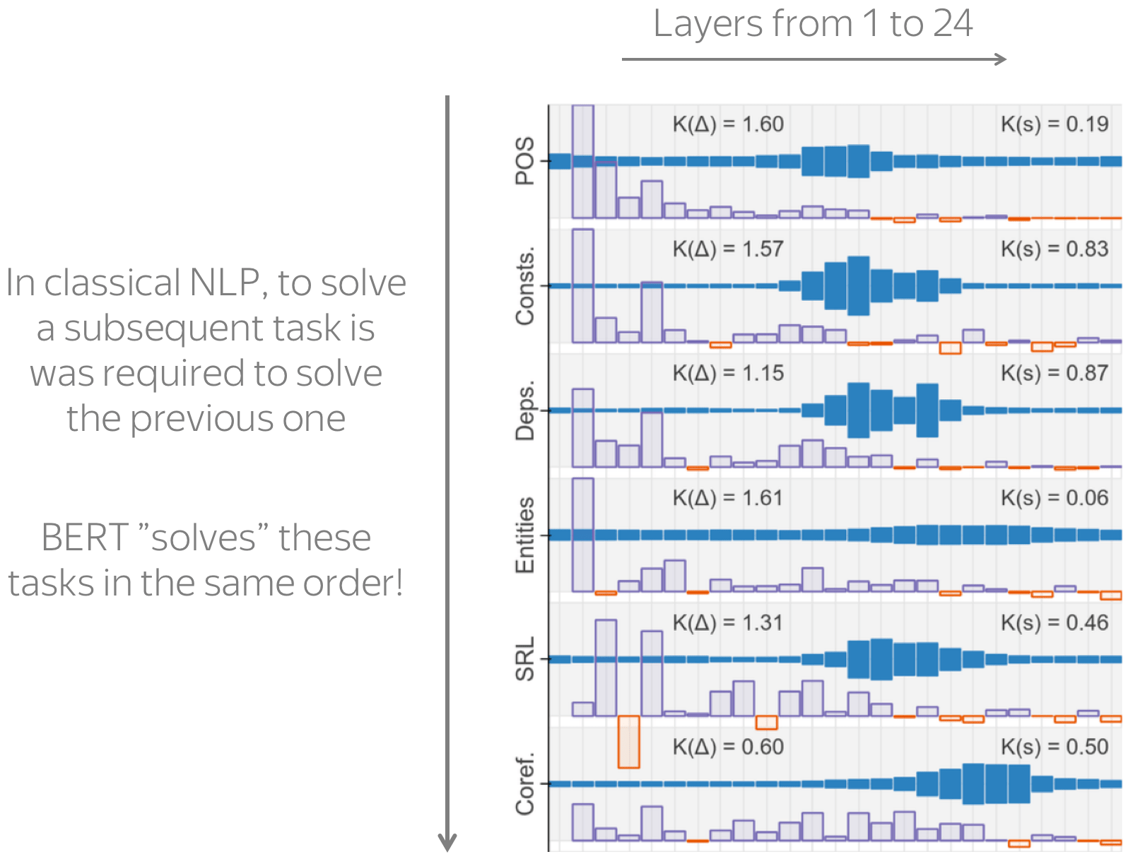
The results are shown in the figure to the right. The layers are shown from left to right, the weights for each layer are shown in dark blue.
We see that as you go from bottom to top layer, a layer's influence for each goes up, then down. But the main result is not in the values per se, but in the way BERT represents different linguistic tasks. In the classical NLP, there was an ordering of different tasks (this is the order shown in the figure and the order in which I showed you the examples for each task). To solve a subsequent task in classical NLP, one had to solve all the previous ones. What is interesting, BERT represents these tasks in the same order! For example, dependencies are represented later than part-of-speech tags, and coreference is learned later than both these tasks.
Looking at Predictions: Do ELMo and BERT Know Facts?
In the Language Modeling lecture, we learned how to evaluate language models for specific phenomena by looking at their predictions. In that lecture, we looked at a very popular subject-verb agreement task. Today, we will do something way more fun - check if a model knows facts! As an example, we use the EMNLP 2019 paper Language Models as Knowledge Bases?.
The figure with the results is from the paper
Language Models as Knowledge Bases?
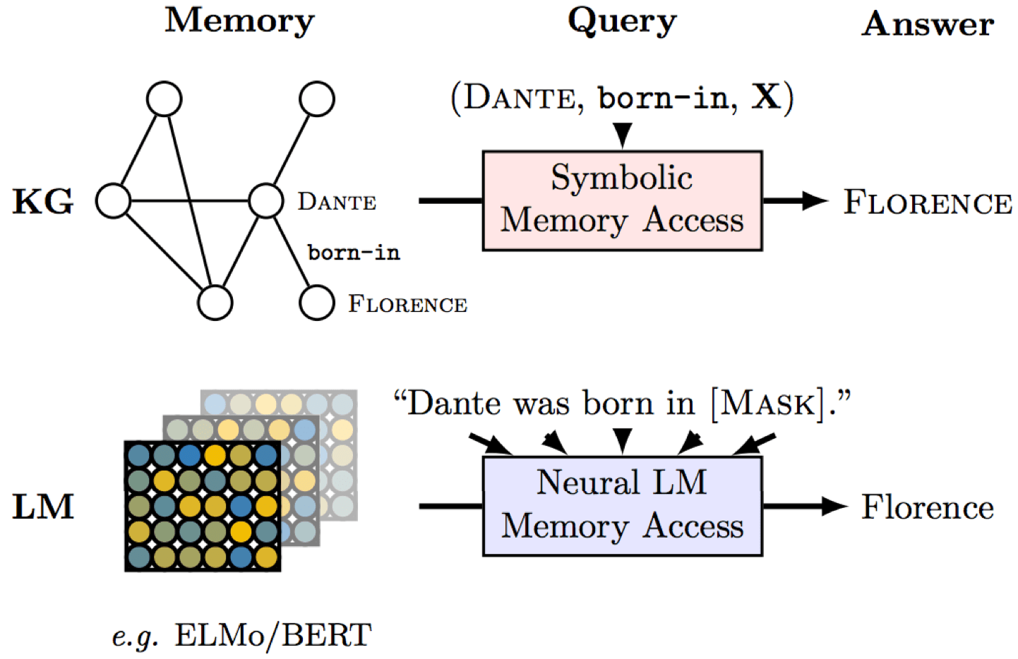
Usually, factual knowledge is stored in knowledge bases that contain triples (subject, relation, object), for example, (Dante, born-in, Florence) as shown in the figure. However, these knowledge bases are hard to obtain: to extract knowledge, one usually has to use complicated pipelines.
But what if pretrained language models (ELMo, BERT) already know the facts? Let's check! Instead of relation triplets, we will feed to a model a cloze-style sentence with a masked object. For example, we give our model a sentence Dante was born in ___ and ask it to predict a token in place of a mask. Note that we do it without any fine-tuning - just a plain language model!
Turns out, pretrained models can know facts quite well. Note that by "know" here we do not mean that they understand anything, but just that the training data statistics captured in these models can be used to extract facts. Look at some examples below (the original paper has more!).
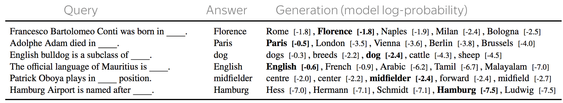
The examples are from the paper
Language Models as Knowledge Bases?
What is more fun, we can look at not only formal facts, but also common knowledge: look at the examples. For more details on the test set construction, see the paper.
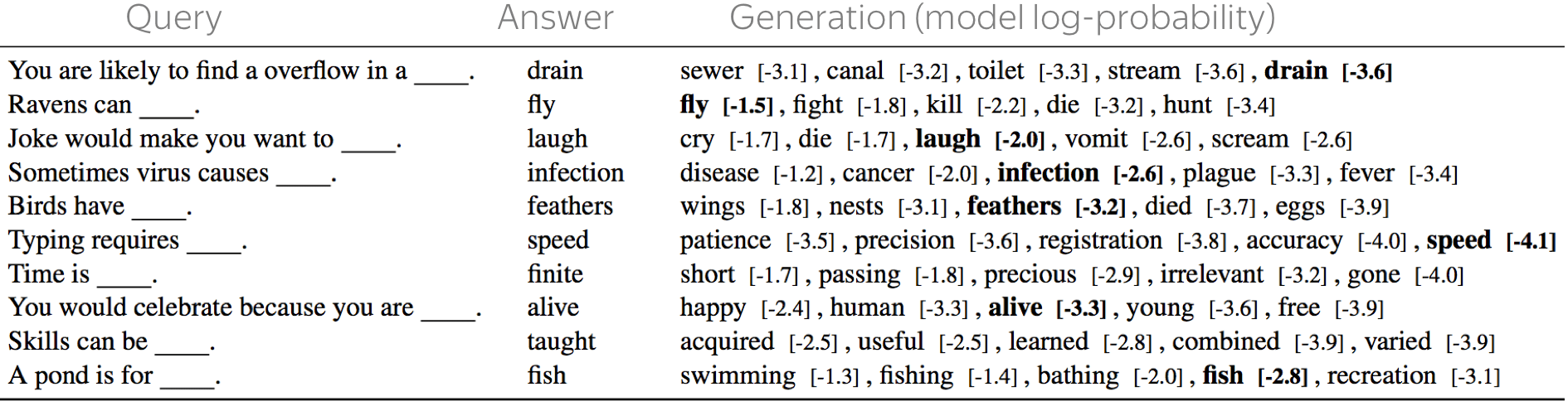
The examples are from the paper
Language Models as Knowledge Bases?
Back to The Key-Value View of FFNs
We saw that BERT and others seem to know some facts. But how are these facts stored in the model? Turns out, some of them are encoded in FFNs!
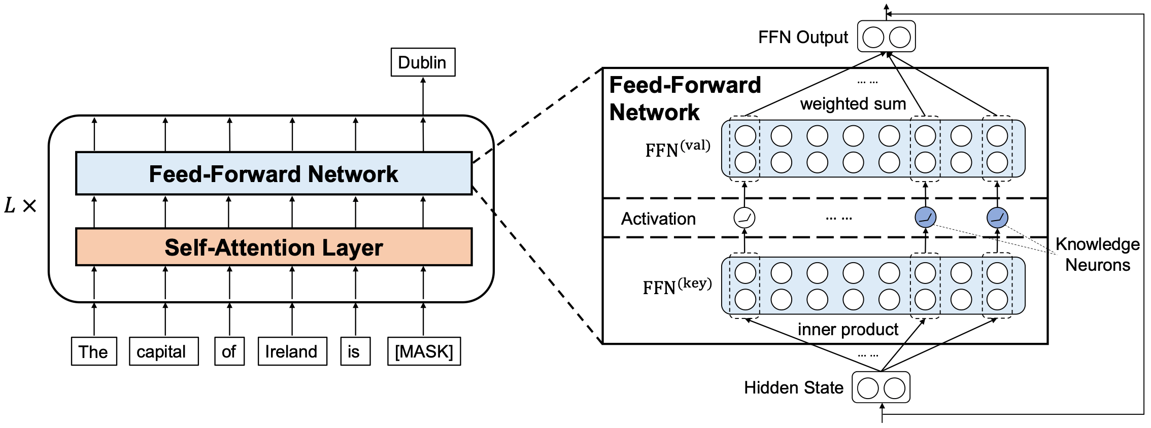
The figure is from the paper
Knowledge Neurons in Pretrained Transformers.
Let us come back to the key-value memory view of FFNs. The paper Knowledge Neurons in Pretrained Transformers looked at (subject, relation) -> object triplets and found that some neurons inside FFNs encode these relations! Specifically, each neuron activates whenever (subject, relation) pair is in the input, and triggers the row that encodes the object.
Research Thinking
Here will be exercises!
This part will be expanding from time to time.

Related Papers
Here will be papers!
The papers will be gradually appearing.

Have Fun!
Coming soon!
We are still working on this!