Sequence to Sequence (seq2seq) and Attention
The most popular sequence-to-sequence task is translation: usually, from one natural language to another. In the last couple of years, commercial systems became surprisingly good at machine translation - check out, for example, Google Translate, Yandex Translate, DeepL Translator, Bing Microsoft Translator. Today we will learn about the core part of these systems.
Except for the popular machine translation between natural languages, you can translate between programming languages (see e.g. the Facebook AI blog post Deep learning to translate between programming languages), or between any sequences of tokens you can come up with. From now on, by machine translation we will mean any general sequence-to-sequence task, i.e. translation between sequences of tokens of any nature.
In the following, we will first learn about the seq2seq basics, then we'll find out about attention - an integral part of all modern systems, and will finally look at the most popular model - Transformer. Of course, with lots of analysis, exercises, papers, and fun!
Sequence to Sequence Basics
Formally, in the machine translation task, we have an input sequence \(x_1, x_2, \dots, x_m\) and an output sequence \(y_1, y_2, \dots, y_n\) (note that their lengths can be different). Translation can be thought of as finding the target sequence that is the most probable given the input; formally, the target sequence that maximizes the conditional probability \(p(y|x)\): \(y^{\ast}=\arg\max\limits_{y}p(y|x).\)
If you are bilingual and can translate between languages easily, you have an intuitive feeling of \(p(y|x)\) and can say something like "...well, this translation is kind of more natural for this sentence". But in machine translation, we learn a function \(p(y|x, \theta)\) with some parameters \(\theta\), and then find its argmax for a given input: \(y'=\arg\max\limits_{y}p(y|x, \theta).\)
To define a machine translation system, we need to answer three questions:
- modeling - how does the model for \(p(y|x, \theta)\) look like?
- learning - how to find the parameters \(\theta\)?
- inference - how to find the best \(y\)?
In this section, we will answer the second and third questions in full, but consider only the simplest model. The more "real" models will be considered later in sections Attention and Transformer.
Encoder-Decoder Framework
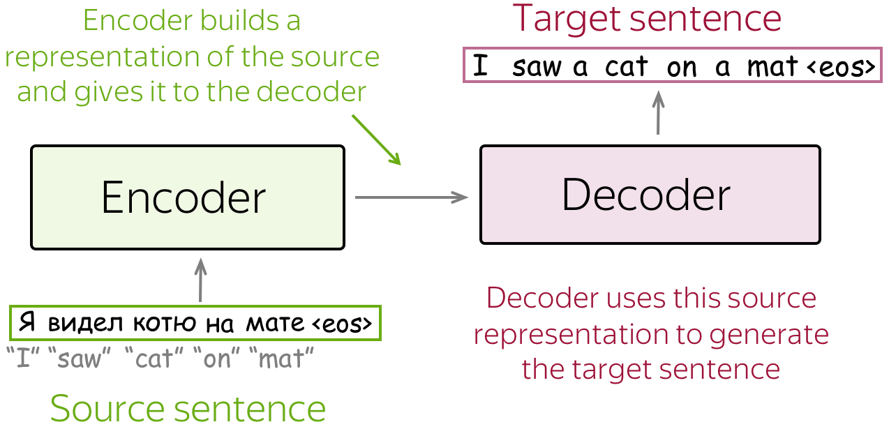
Encoder-decoder is the standard modeling paradigm for sequence-to-sequence tasks. This framework consists of two components:
- encoder - reads source sequence and produces its representation;
- decoder - uses source representation from the encoder to generate the target sequence.
In this lecture, we'll see different models, but they all have this encoder-decoder structure.
Conditional Language Models
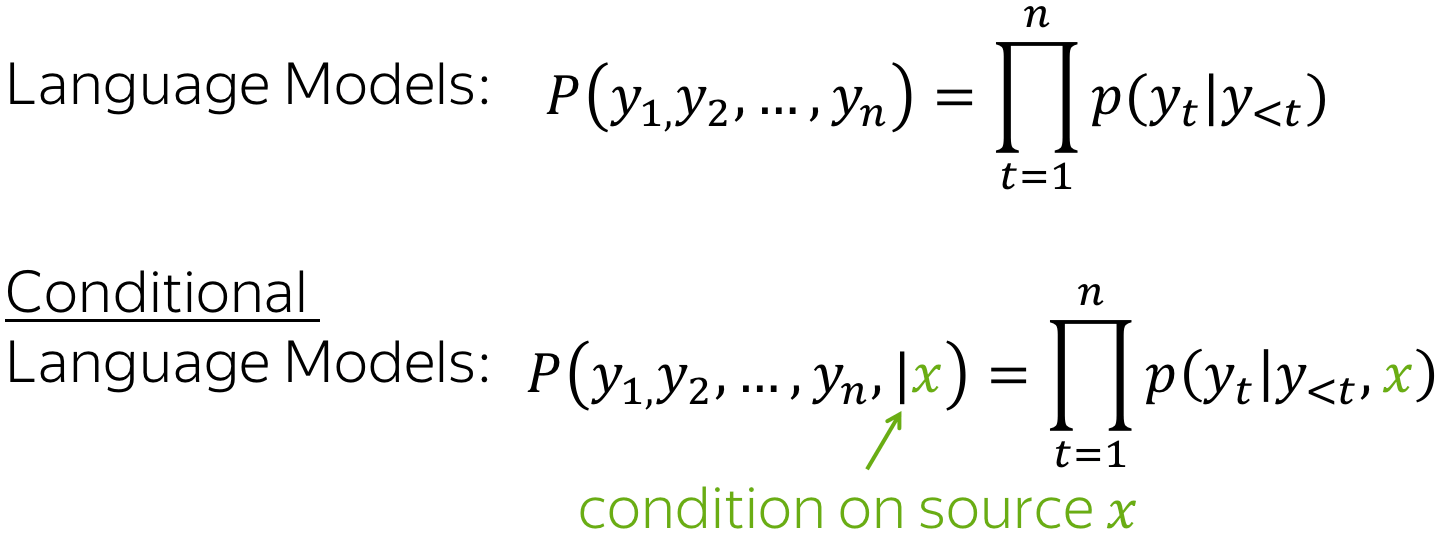
In the Language Modeling lecture, we learned to estimate the probability \(p(y)\) of sequences of tokens \(y=(y_1, y_2, \dots, y_n)\). While language models estimate the unconditional probability \(p(y)\) of a sequence \(y\), sequence-to-sequence models need to estimate the conditional probability p(y|x) of a sequence \(y\) given a source \(x\). That's why sequence-to-sequence tasks can be modeled as Conditional Language Models (CLM) - they operate similarly to LMs, but additionally receive source information \(x\).
Lena: Note that Conditional Language Modeling is something more than just a way to solve sequence-to-sequence tasks. In the most general sense, \(x\) can be something other than a sequence of tokens. For example, in the Image Captioning task, \(x\) is an image and \(y\) is a description of this image.
Since the only difference from LMs is the presence of source \(x\), the modeling and training is very similar to language models. In particular, the high-level pipeline is as follows:
- feed source and previously generated target words into a network;
- get vector representation of context (both source and previous target) from the networks decoder;
- from this vector representation, predict a probability distribution for the next token.
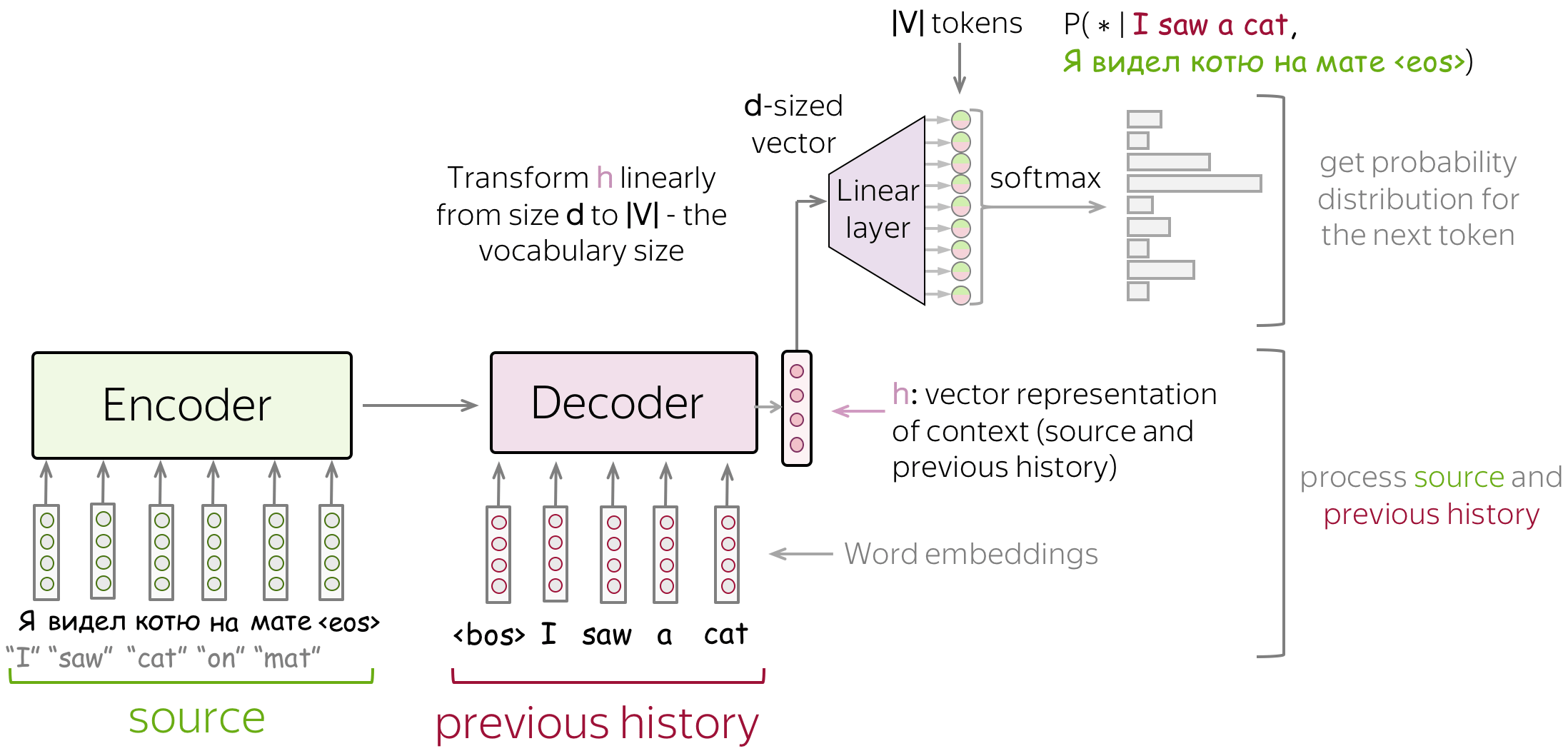
Similarly to neural classifiers and language models, we can think about the classification part (i.e., how to get token probabilities from a vector representation of a text) in a very simple way. Vector representation of a text has some dimensionality \(d\), but in the end, we need a vector of size \(|V|\) (probabilities for \(|V|\) tokens/classes). To get a \(|V|\)-sized vector from a \(d\)-sized, we can use a linear layer. Once we have a \(|V|\)-sized vector, all is left is to apply the softmax operation to convert the raw numbers into token probabilities.
The Simplest Model: Two RNNs for Encoder and Decoder
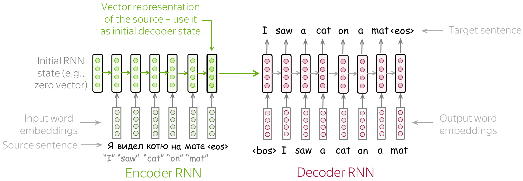
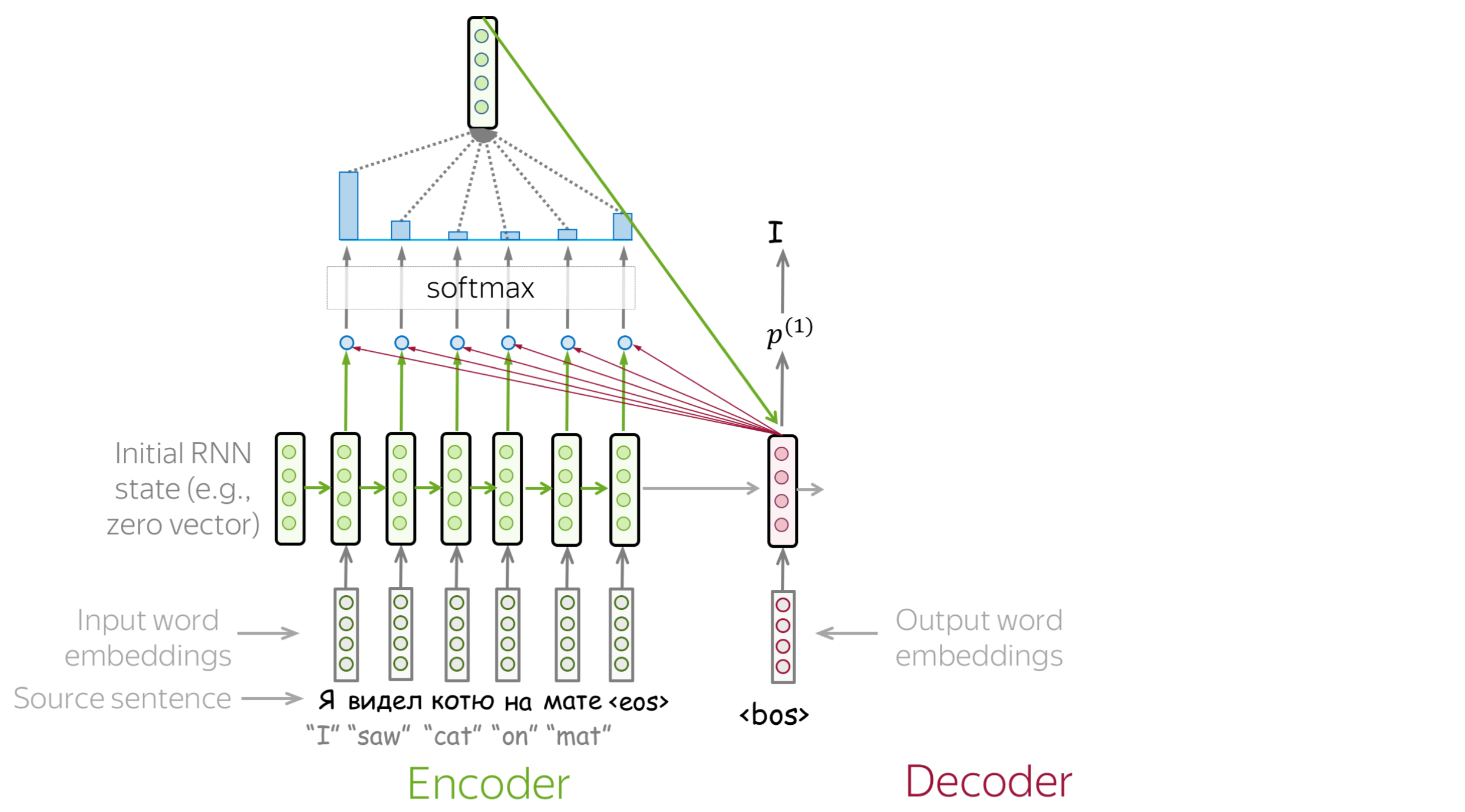
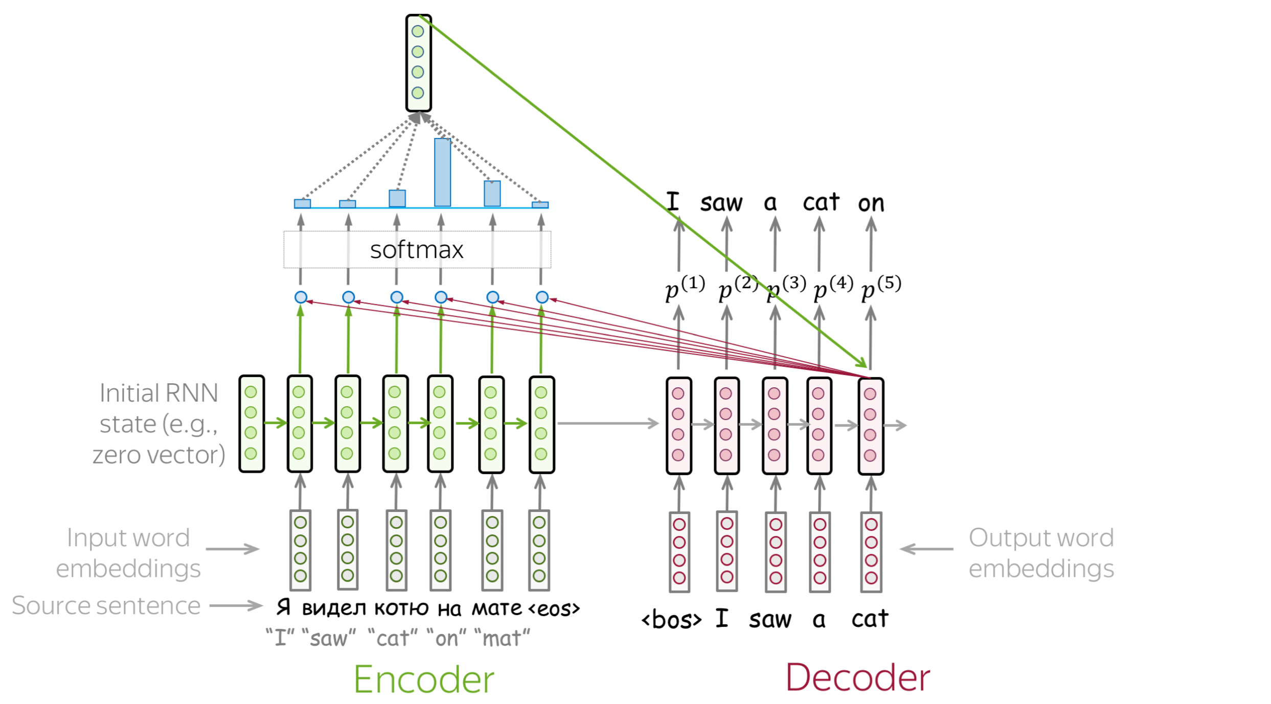
The simplest encoder-decoder model consists of two RNNs (LSTMs): one for the encoder and another for the decoder. Encoder RNN reads the source sentence, and the final state is used as the initial state of the decoder RNN. The hope is that the final encoder state "encodes" all information about the source, and the decoder can generate the target sentence based on this vector.
This model can have different modifications: for example, the encoder and decoder can have several layers. Such a model with several layers was used, for example, in the paper Sequence to Sequence Learning with Neural Networks - one of the first attempts to solve sequence-to-sequence tasks using neural networks.
In the same paper, the authors looked at the last encoder state and visualized several examples - look below. Interestingly, representations of sentences with similar meaning but different structure are close!
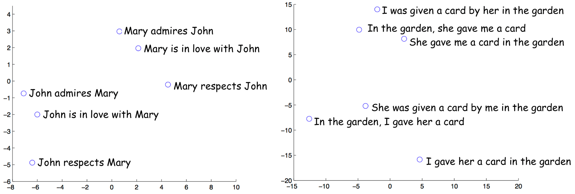
The examples are from the paper
Sequence to Sequence Learning with Neural Networks.
The paper Sequence to Sequence Learning with Neural Networks introduced an elegant trick to make such a simple LSTM model work better. Learn more in this exercise in the Research Thinking section.
Training: The Cross-Entropy Loss (Once Again)
Lena: This is the same cross-entropy loss we discussed before in the Text Classification and in the Language Modeling lectures - you can skip this part or go through it quite easily :)
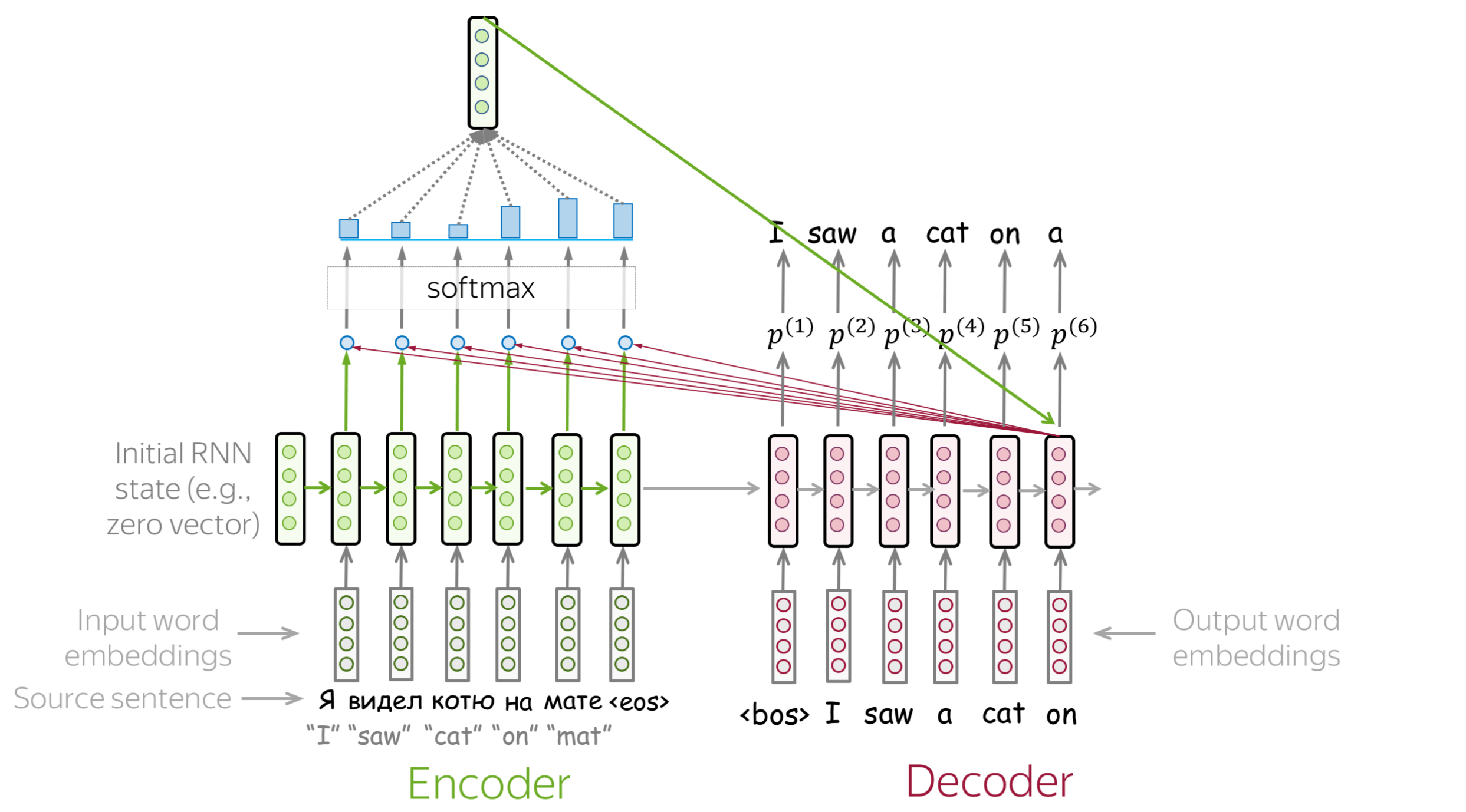
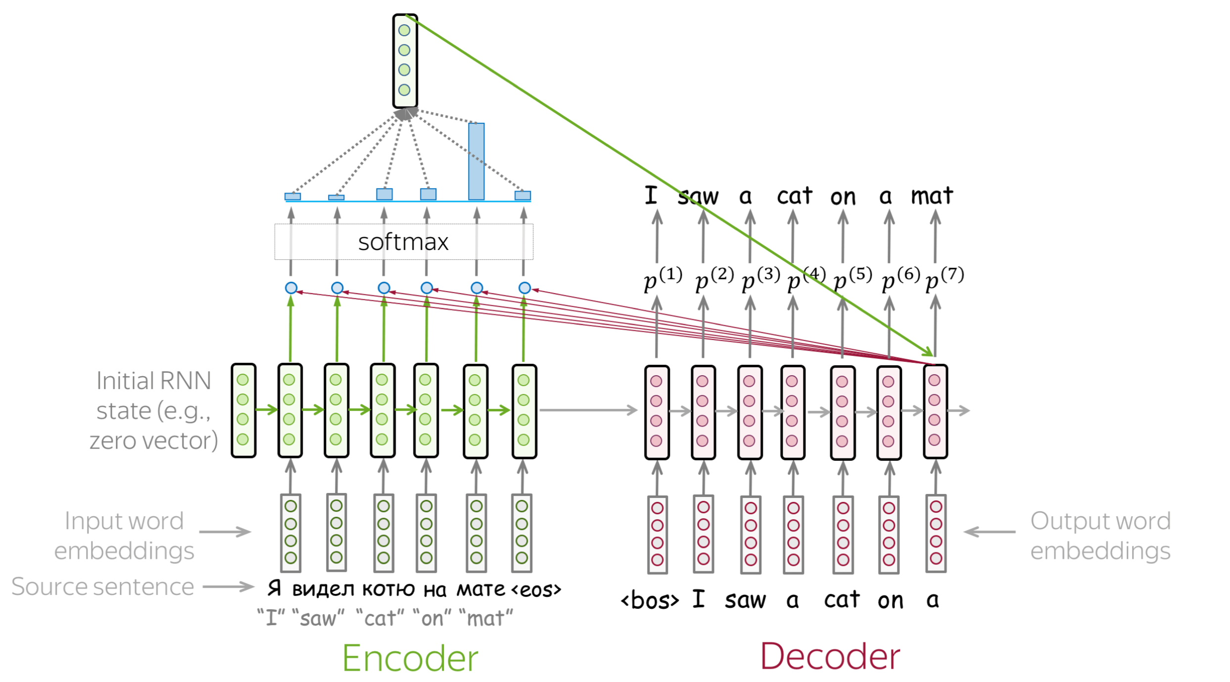
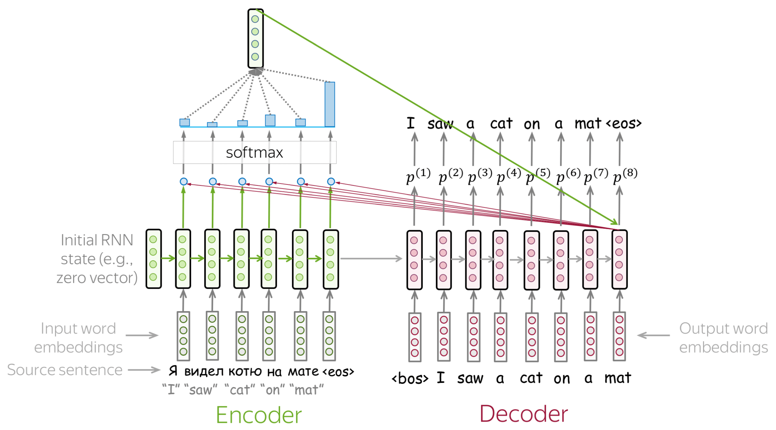
Similarly to neural LMs, neural seq2seq models are trained to predict probability distributions of the next token given previous context (source and previous target tokens). Intuitively, at each step we maximize the probability a model assigns to the correct token.
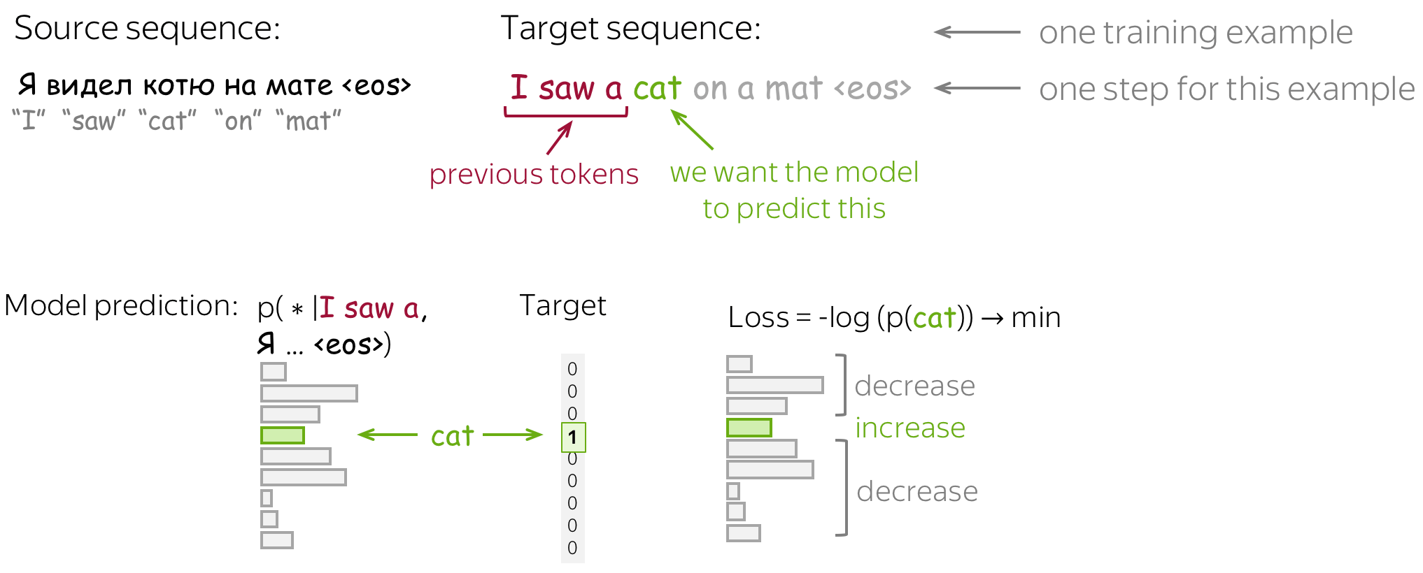
Formally, let's assume we have a training instance with the source \(x=(x_1, \dots, x_m)\) and the target \(y=(y_1, \dots, y_n)\). Then at the timestep \(t\), a model predicts a probability distribution \(p^{(t)} = p(\ast|y_1, \dots, y_{t-1}, x_1, \dots, x_m)\). The target at this step is \(p^{\ast}=\mbox{one-hot}(y_t)\), i.e., we want a model to assign probability 1 to the correct token, \(y_t\), and zero to the rest.
The standard loss function is the cross-entropy loss. Cross-entropy loss for the target distribution \(p^{\ast}\) and the predicted distribution \(p^{}\) is \[Loss(p^{\ast}, p^{})= - p^{\ast} \log(p) = -\sum\limits_{i=1}^{|V|}p_i^{\ast} \log(p_i).\] Since only one of \(p_i^{\ast}\) is non-zero (for the correct token \(y_t\)), we will get \[Loss(p^{\ast}, p) = -\log(p_{y_t})=-\log(p(y_t| y_{\mbox{<}t}, x)).\] At each step, we maximize the probability a model assigns to the correct token. Look at the illustration for a single timestep.
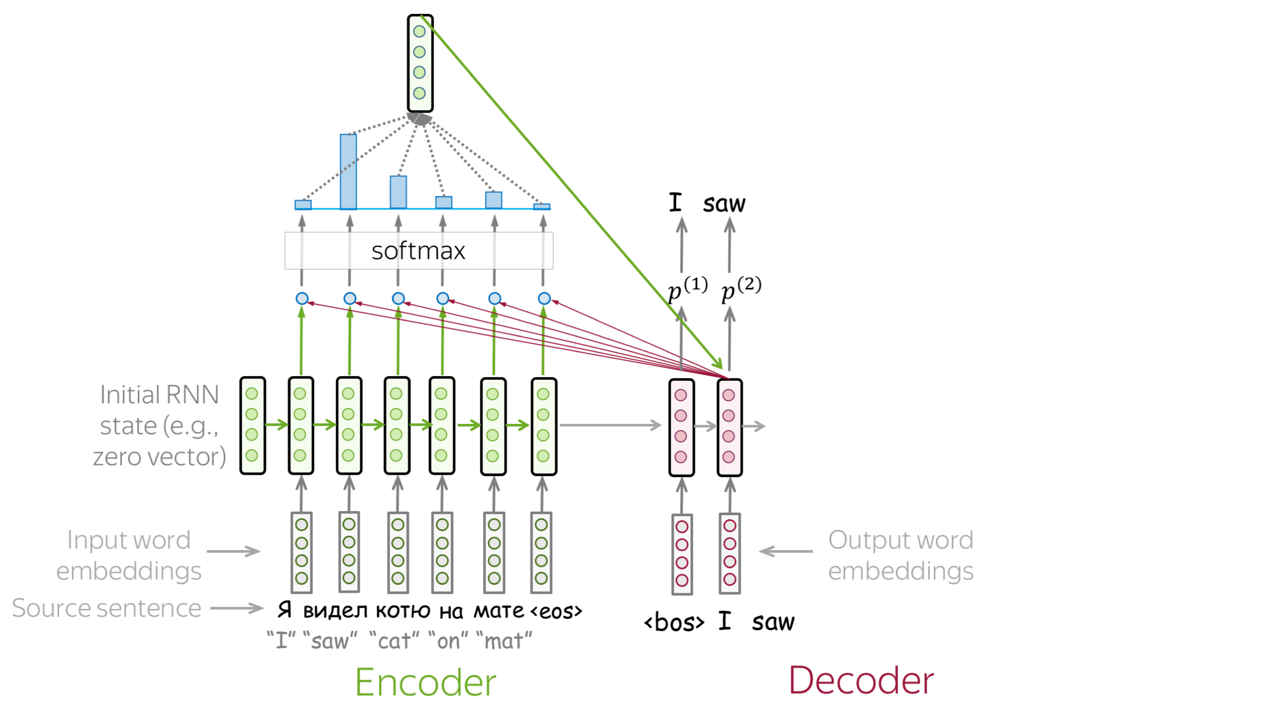
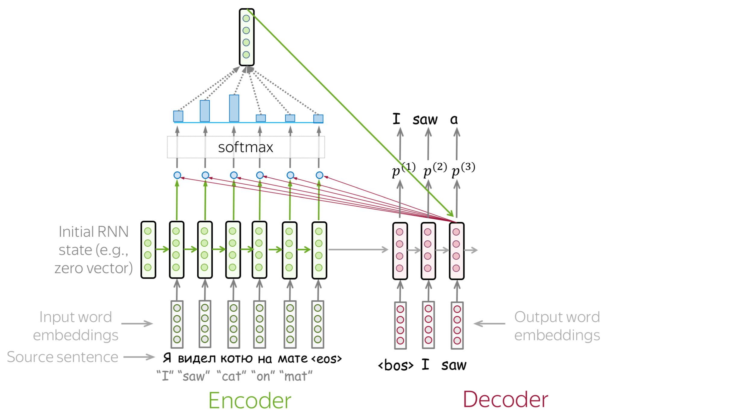
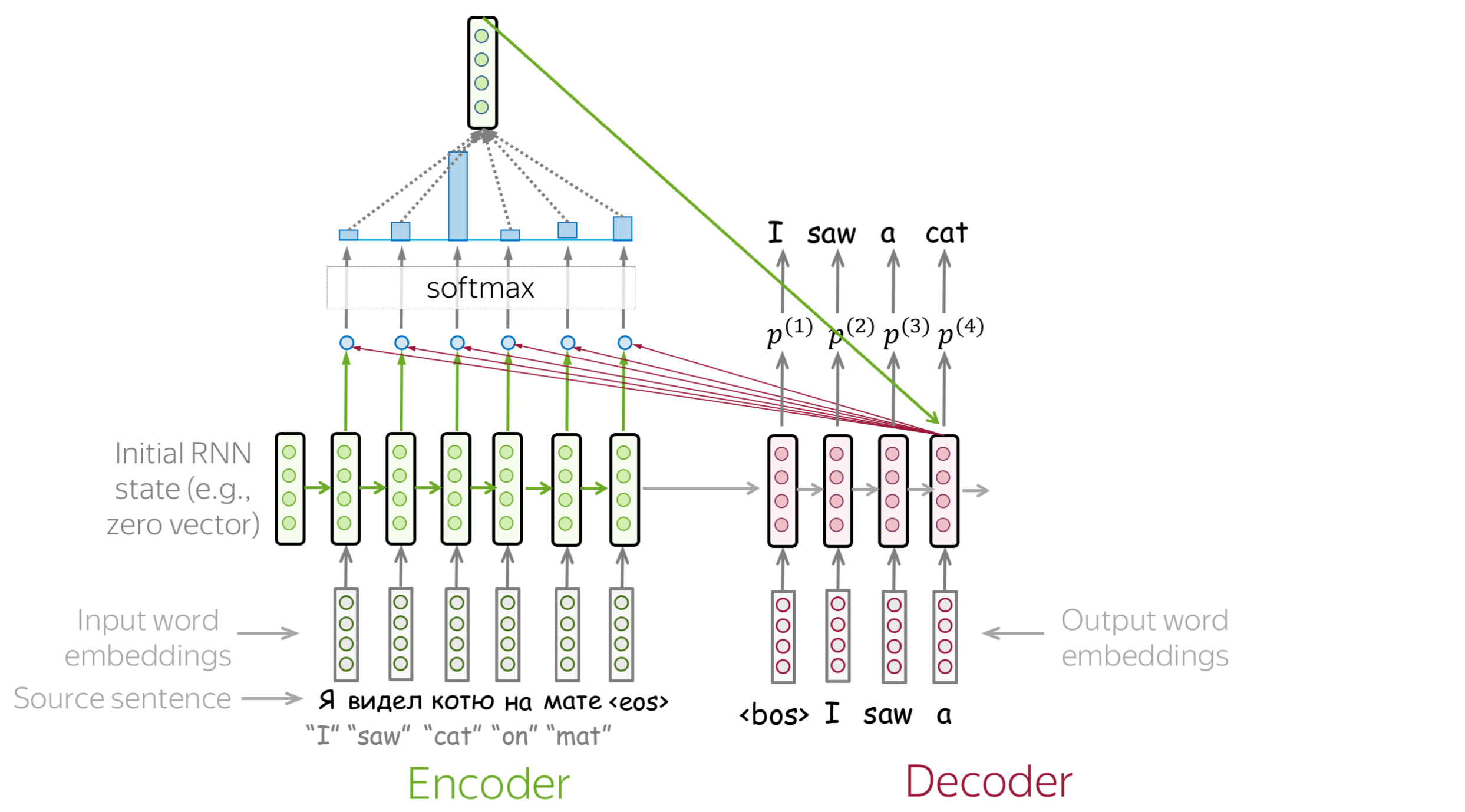
For the whole example, the loss will be \(-\sum\limits_{t=1}^n\log(p(y_t| y_{\mbox{<}t}, x))\). Look at the illustration of the training process (the illustration is for the RNN model, but the model can be different).
Inference: Greedy Decoding and Beam Search
Now when we understand how a model can look like and how to train this model, let's think how to generate a translation using this model. We model the probability of a sentence as follows:
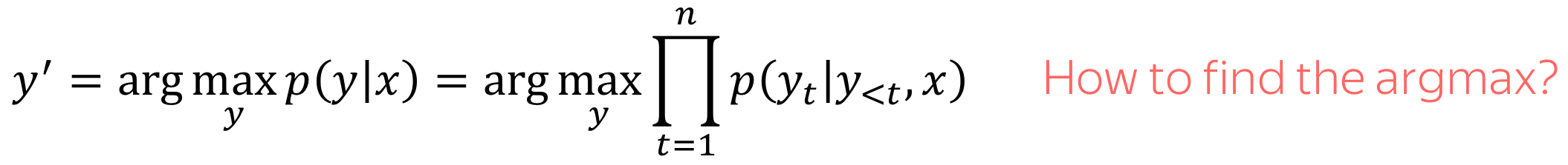
Now the main question is: how to find the argmax?
Note that we can not find the exact solution. The total number of hypotheses we need to check is \(|V|^n\), which is not feasible in practice. Therefore, we will find an approximate solution.
Lena: In reality, the exact solution is usually worse than the approximate ones we will be using.
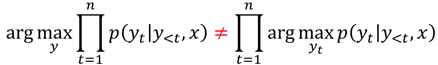
• Greedy Decoding: At each step, pick the most probable token
The straightforward decoding strategy is greedy - at each step, generate a token with the highest probability. This can be a good baseline, but this method is inherently flawed: the best token at the current step does not necessarily lead to the best sequence.
• Beam Search: Keep track of several most probably hypotheses
Instead, let's keep several hypotheses. At each step, we will be continuing each of the current hypotheses and pick top-N of them. This is called beam search.
Usually, the beam size is 4-10. Increasing beam size is computationally inefficient and, what is more important, leads to worse quality.
Attention
The Problem of Fixed Encoder Representation
Problem: Fixed source representation is suboptimal: (i) for the encoder, it is hard to compress the sentence; (ii) for the decoder, different information may be relevant at different steps.
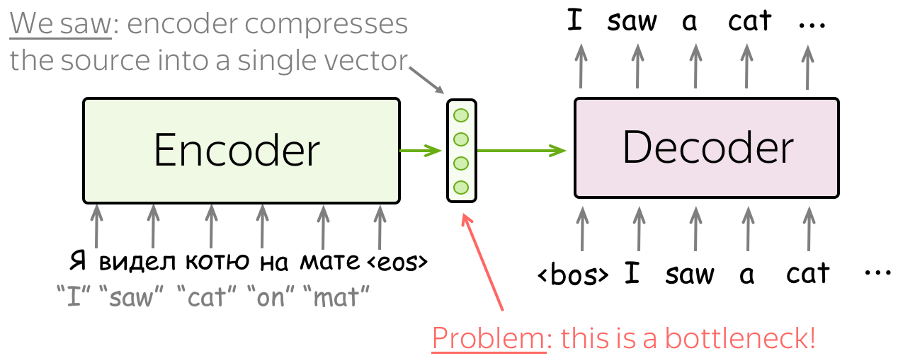
In the models we looked at so far, the encoder compressed the whole source sentence into a single vector. This can be very hard - the number of possible source sentences (hence, their meanings) is infinite. When the encoder is forced to put all information into a single vector, it is likely to forget something.
Lena: Imagine the whole universe in all its beauty - try to visualize everything you can find there and how you can describe it in words. Then imagine all of it is compressed into a single vector of size e.g. 512. Do you feel that the universe is still ok?
Not only it is hard for the encoder to put all information into a single vector - this is also hard for the decoder. The decoder sees only one representation of source. However, at each generation step, different parts of source can be more useful than others. But in the current setting, the decoder has to extract relevant information from the same fixed representation - hardly an easy thing to do.
Attention: A High-Level View
Attention was introduced in the paper Neural Machine Translation by Jointly Learning to Align and Translate to address the fixed representation problem.
Attention: At different steps, let a model "focus" on different parts of the input.
An attention mechanism is a part of a neural network. At each decoder step, it decides which source parts are more important. In this setting, the encoder does not have to compress the whole source into a single vector - it gives representations for all source tokens (for example, all RNN states instead of the last one).
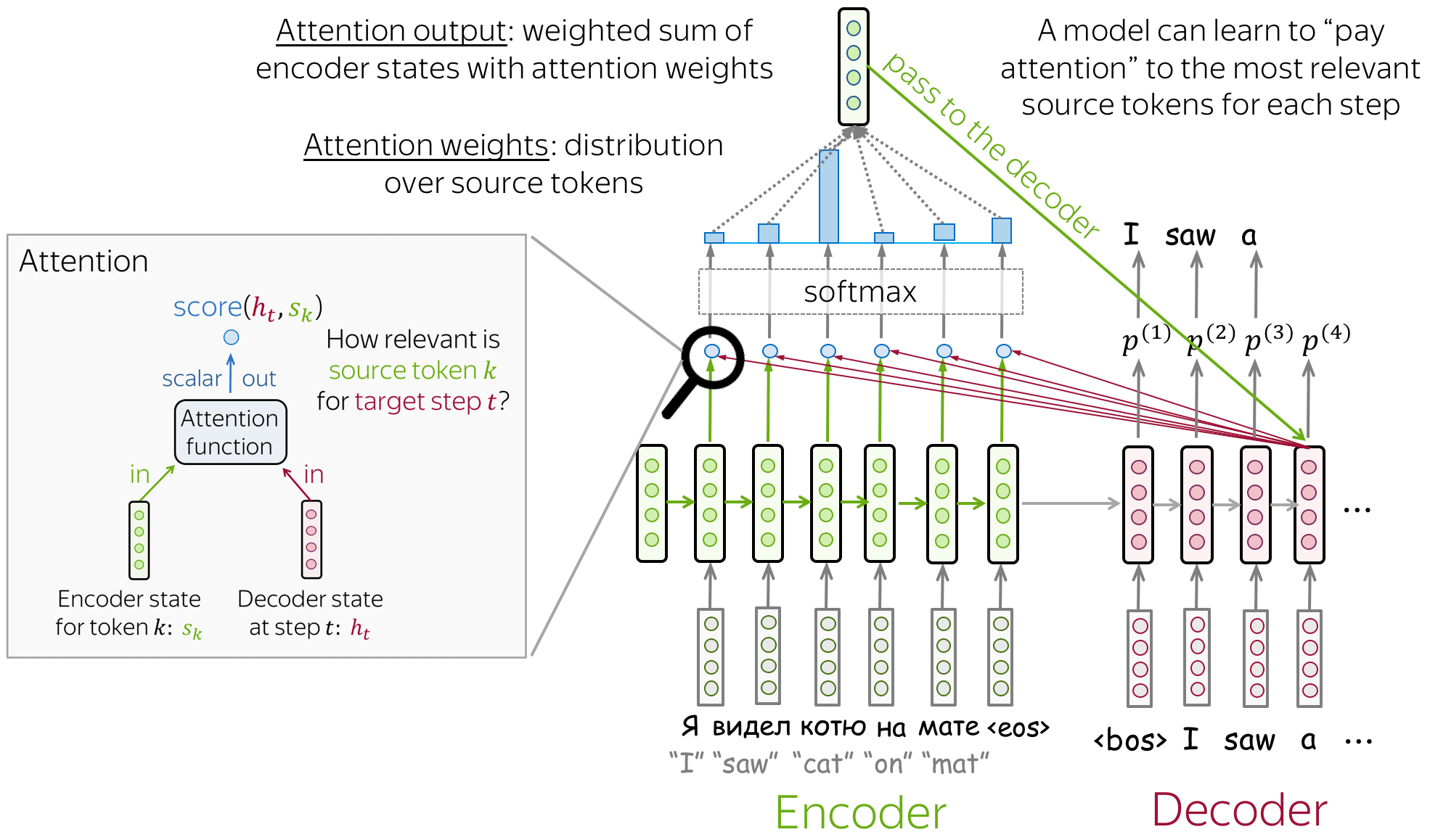
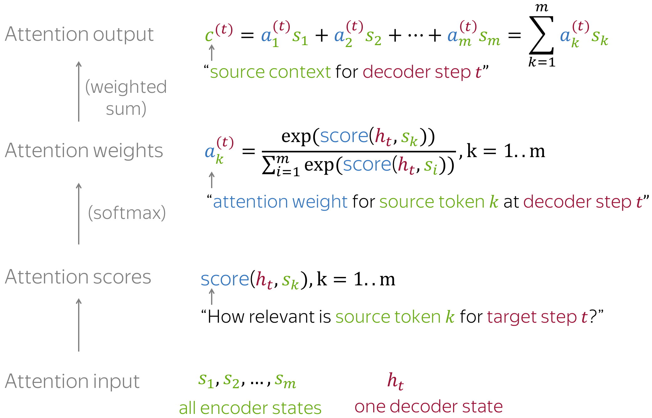
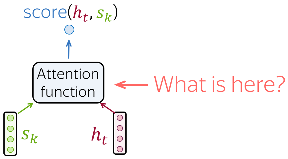
At each decoder step, attention
- receives attention input: a decoder state \(\color{#b01277}{h_t}\) and all encoder states \(\color{#7fb32d}{s_1}\), \(\color{#7fb32d}{s_2}\), ..., \(\color{#7fb32d}{s_m}\);
- computes attention scores
For each encoder state \(\color{#7fb32d}{s_k}\), attention computes its "relevance" for this decoder state \(\color{#b01277}{h_t}\). Formally, it applies an attention function which receives one decoder state and one encoder state and returns a scalar value \(\color{#307cc2}{score}(\color{#b01277}{h_t}\color{black}{,}\color{#7fb32d}{s_k}\color{black})\); - computes attention weights: a probability distribution - softmax applied to attention scores;
- computes attention output: the weighted sum of encoder states with attention weights.
The general computation scheme is shown below.
Note: Everything is differentiable - learned end-to-end!
The main idea that a network can learn which input parts are more important at each step. Since everything here is differentiable (attention function, softmax, and all the rest), a model with attention can be trained end-to-end. You don't need to specifically teach the model to pick the words you want - the model itself will learn to pick important information.
How to: go over the slides at your pace. Try to notice how attention weights change from step to step - which words are the most important at each step?
How to Compute Attention Score?
In the general pipeline above, we haven't specified how exactly we compute attention scores. You can apply any function you want - even a very complicated one. However, usually you don't need to - there are several popular and simple variants which work quite well.
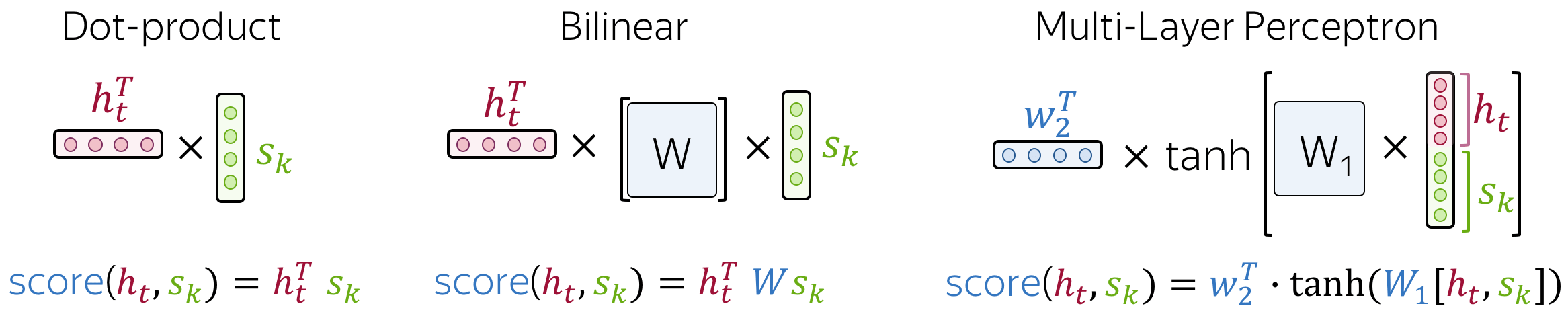
The most popular ways to compute attention scores are:
- dot-product - the simplest method;
- bilinear function (aka "Luong attention") - used in the paper Effective Approaches to Attention-based Neural Machine Translation;
- multi-layer perceptron (aka "Bahdanau attention") - the method proposed in the original paper.
Model Variants: Bahdanau and Luong
When talking about the early attention models, you are most likely to hear these variants:
- Bahdanau attention - from the paper Neural Machine Translation by Jointly Learning to Align and Translate by Dzmitry Bahdanau, KyungHyun Cho and Yoshua Bengio (this is the paper that introduced the attention mechanism for the first time);
- Luong attention - from the paper Effective Approaches to Attention-based Neural Machine Translation by Minh-Thang Luong, Hieu Pham, Christopher D. Manning.
These may refer to either score functions of the whole models used in these papers. In this part, we will look more closely at these two model variants.
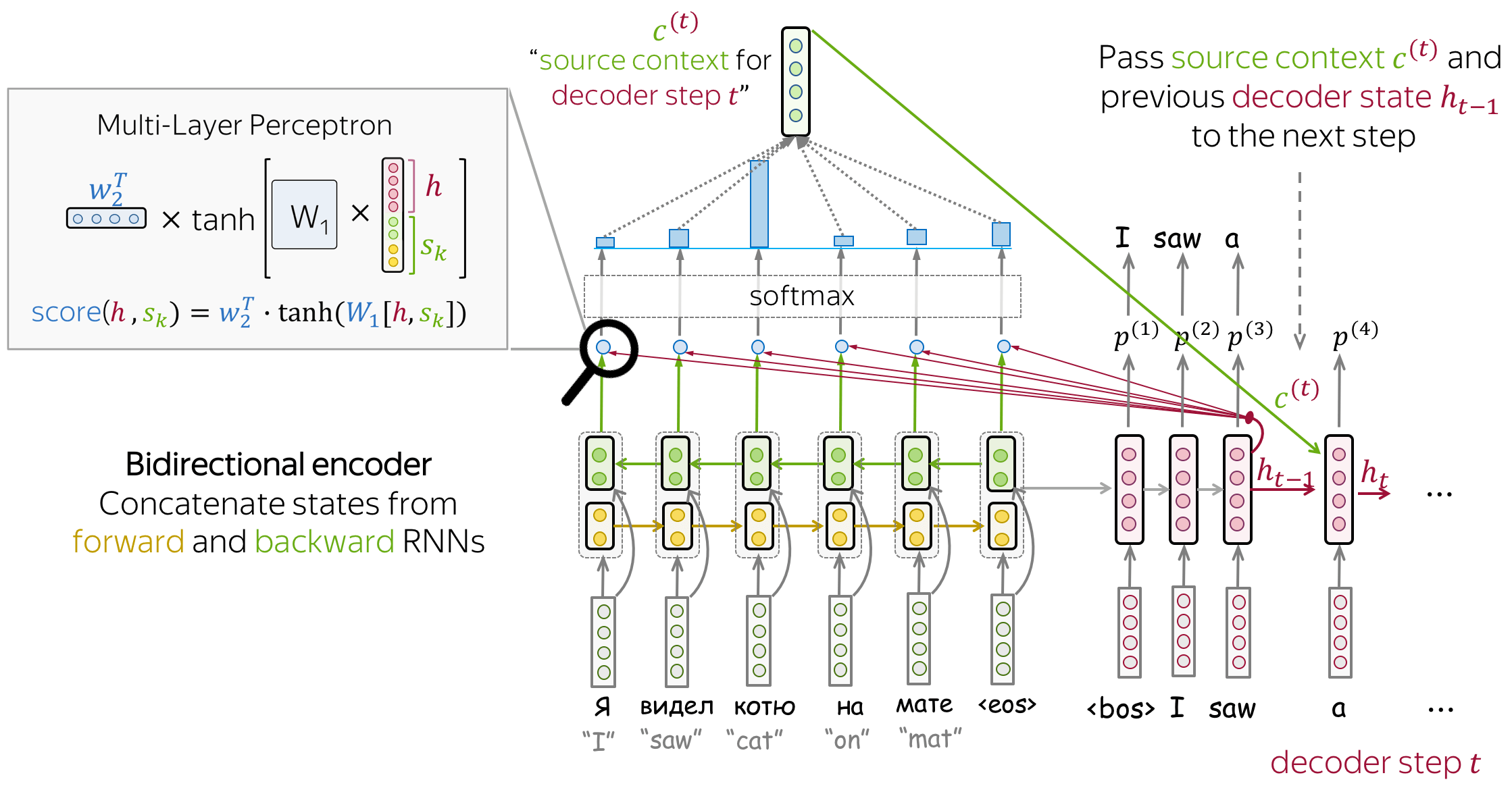
Bahdanau Model
- encoder: bidirectional
To better encode each source word, the encoder has two RNNs, forward and backward, which read input in the opposite directions. For each token, states of the two RNNs are concatenated. - attention score: multi-layer perceptron
To get an attention score, apply a multi-layer perceptron (MLP) to an encoder state and a decoder state. - attention applied: between decoder steps
Attention is used between decoder steps: state \(\color{#b01277}{h_{t-1}}\) is used to compute attention and its output \(\color{#7fb32d}{c}^{\color{#b01277}{(t)}}\), and both \(\color{#b01277}{h_{t-1}}\) and \(\color{#7fb32d}{c}^{\color{#b01277}{(t)}}\) are passed to the decoder at step \(t\).
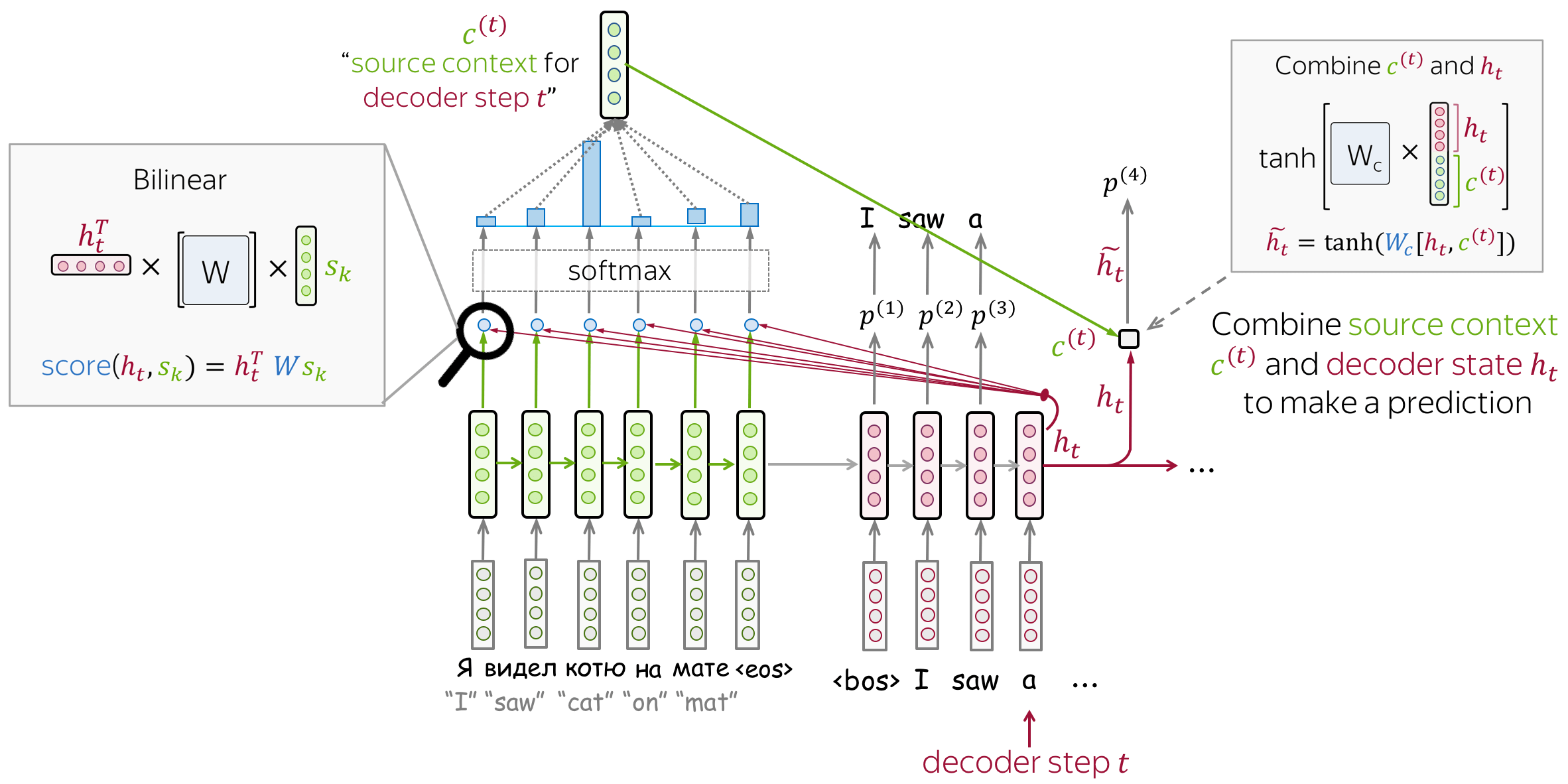
Luong Model
While the paper considers several model variants, the one which is usually called "Luong attention" is the following:
- encoder: unidirectional (simple)
- attention score: bilinear function
- attention applied: between decoder RNN state \(t\) and prediction for this step
Attention is used after RNN decoder step \(t\) before making a prediction. State \(\color{#b01277}{h_{t}}\) used to compute attention and its output \(\color{#7fb32d}{c}^{\color{#b01277}{(t)}}\). Then \(\color{#b01277}{h_{t}}\) is combined with \(\color{#7fb32d}{c}^{\color{#b01277}{(t)}}\) to get an updated representation \(\color{#b01277}{\tilde{h}_{t}}\), which is used to get a prediction.
Attention Learns (Nearly) Alignment
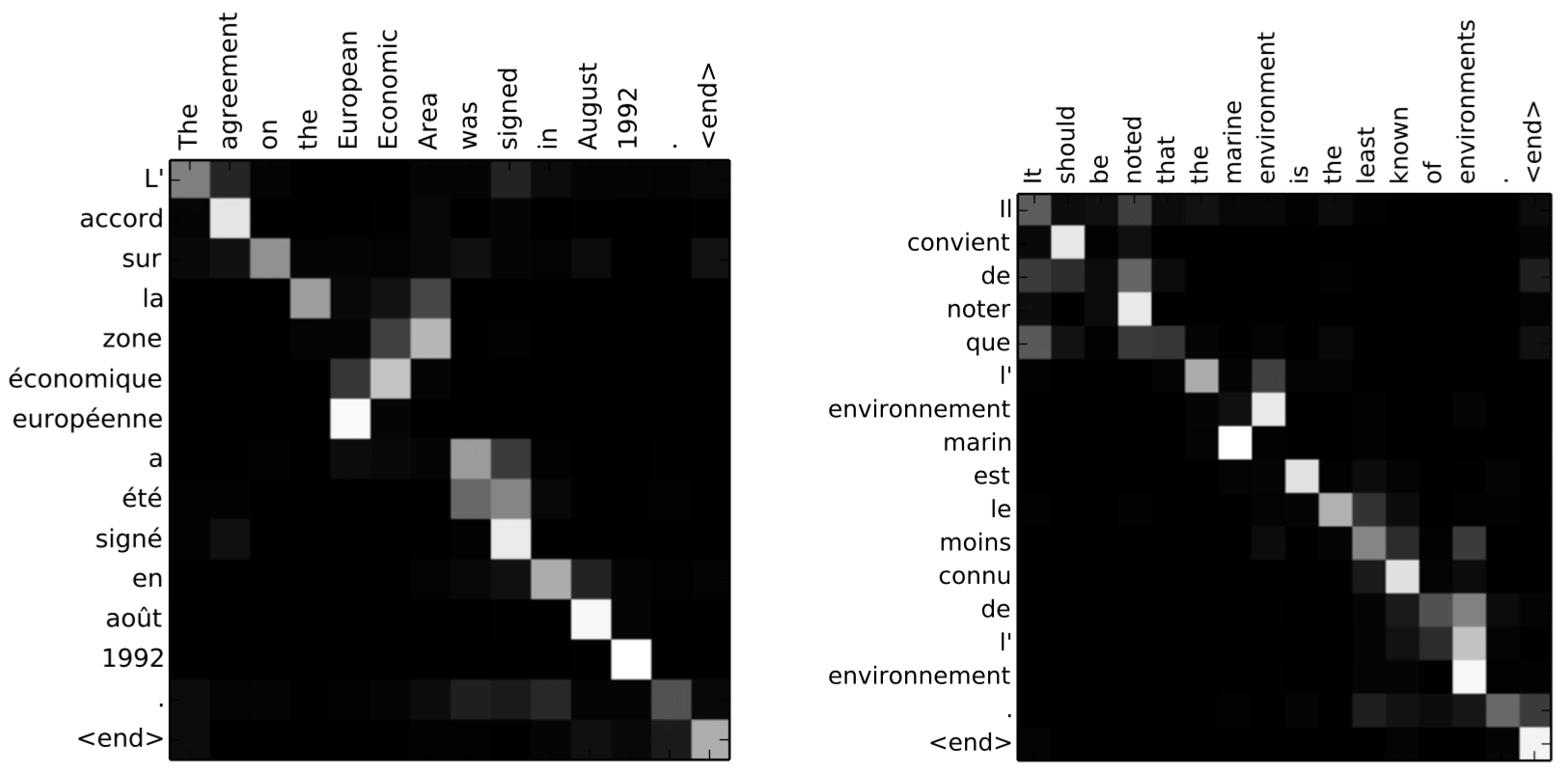
Remember the motivation for attention? At different steps, the decoder may need to focus on different source tokens, the ones which are more relevant at this step. Let's look at attention weights - which source words does the decoder use?
The examples are from the paper
Neural Machine Translation
by Jointly Learning to Align and Translate.
From the examples, we see that attention learned (soft) alignment between source and target words - the decoder looks at those source tokens which it is translating at the current step.
Lena: "Alignment" is a term from statistical machine translation, but in this part, its intuitive understanding as "what is translated to what" is enough.
Transformer: Attention is All You Need
Transformer is a model introduced in the paper Attention is All You Need in 2017. It is based solely on attention mechanisms: i.e., without recurrence or convolutions. On top of higher translation quality, the model is faster to train by up to an order of magnitude. Currently, Transformers (with variations) are de-facto standard models not only in sequence to sequence tasks but also for language modeling and in pretraining settings, which we consider in the next lecture.
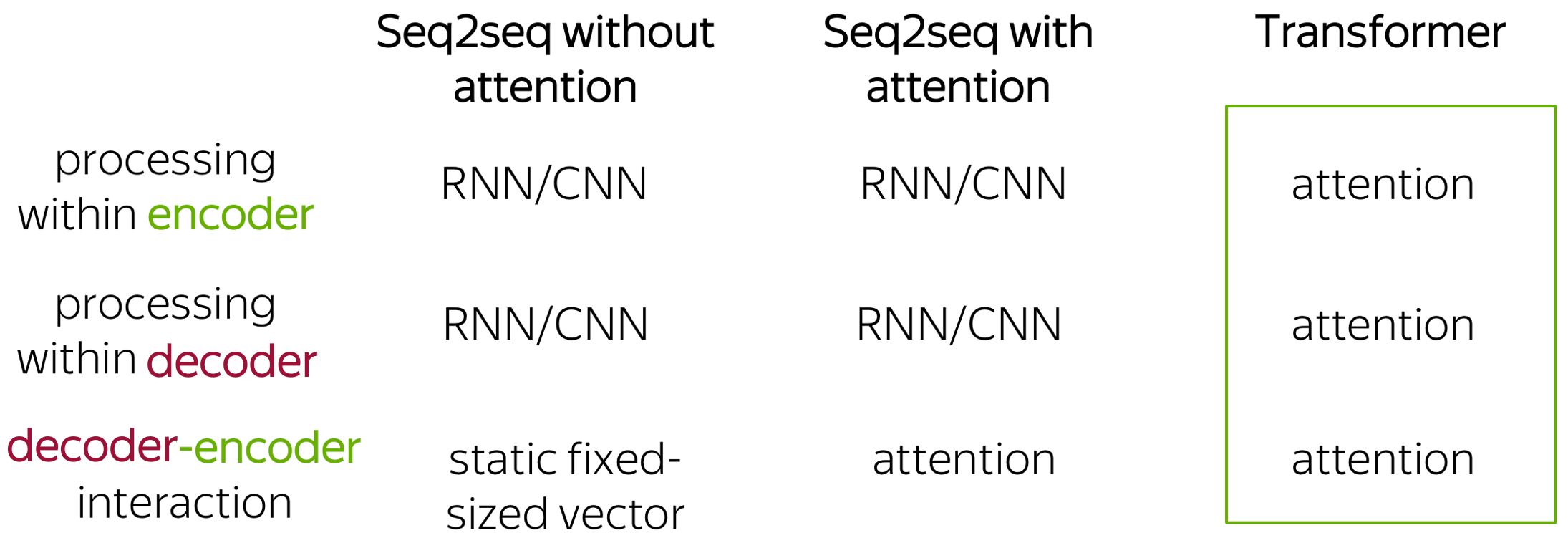
Transformer introduced a new modeling paradigm: in contrast to previous models where processing within encoder and decoder was done with recurrence or convolutions, Transformer operates using only attention.
Look at the illustration from the Google AI blog post introducing Transformer.
![]()
The animation is from the
Google AI blog post.
Without going into too many details, let's put into words what just saw in the illustration. We'll get something like the following:
Ok, but are there any reasons why this can be more suitable that RNNs for language understanding? Let's look at the example.
When encoding a sentence, RNNs won't understand what bank means until they read the whole sentence, and this can take a while for long sequences. In contrast, in Transformer's encoder tokens interact with each other all at once.
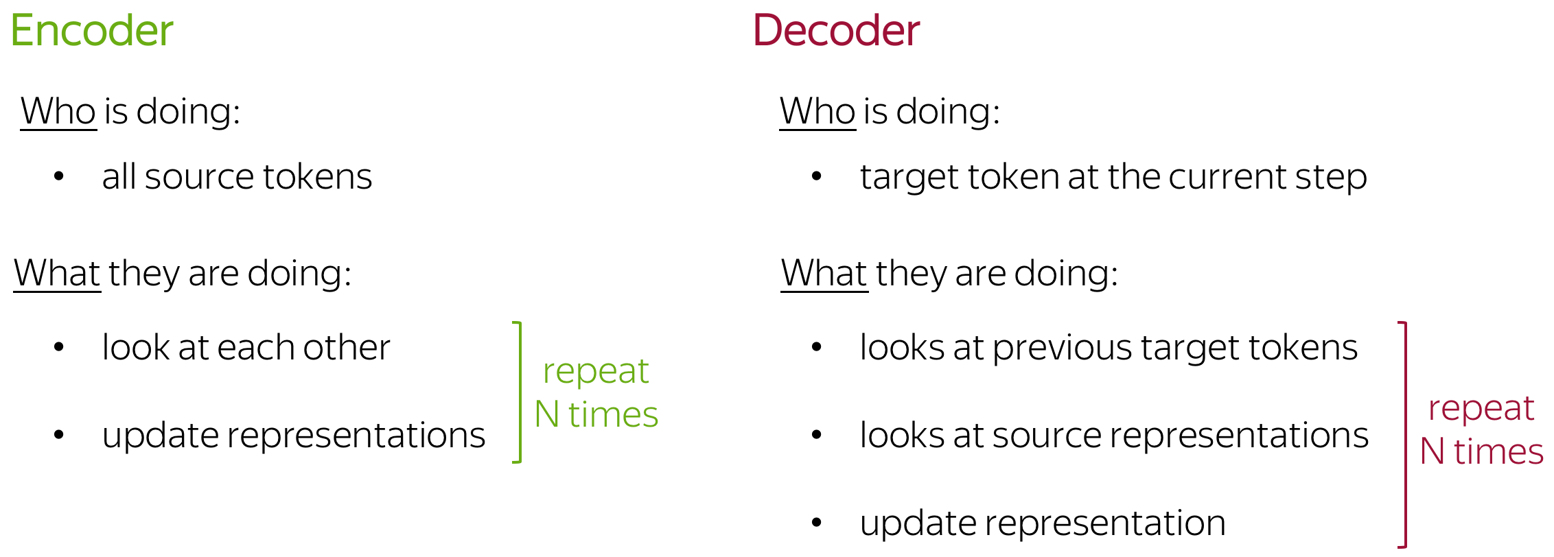
Intuitively, Transformer's encoder can be thought of as a sequence of reasoning steps (layers). At each step, tokens look at each other (this is where we need attention - self-attention), exchange information and try to understand each other better in the context of the whole sentence. This happens in several layers (e.g., 6).
In each decoder layer, tokens of the prefix also interact with each other via a self-attention mechanism, but additionally, they look at the encoder states (without this, no translation can happen, right?).
Now, let's try to understand how exactly this is implemented in the model.
Self-Attention: the "Look at Each Other" Part
Self-attention is one of the key components of the model. The difference between attention and self-attention is that self-attention operates between representations of the same nature: e.g., all encoder states in some layer.
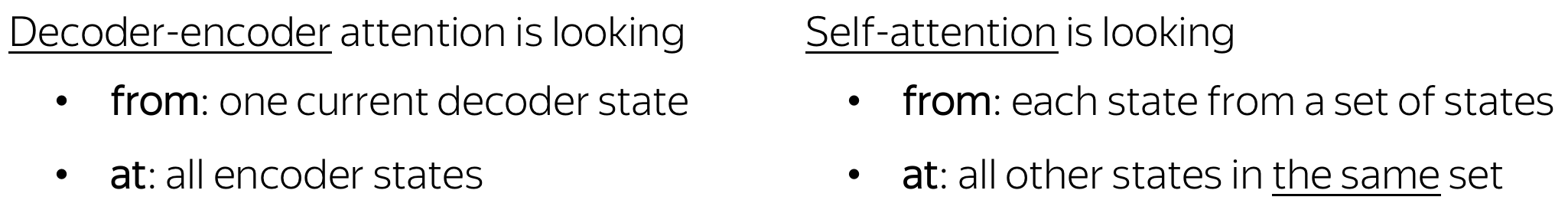
Self-attention is the part of the model where tokens interact with each other. Each token "looks" at other tokens in the sentence with an attention mechanism, gathers context, and updates the previous representation of "self". Look at the illustration.
Note that in practice, this happens in parallel.
Query, Key, and Value in Self-Attention
Formally, this intuition is implemented with a query-key-value attention. Each input token in self-attention receives three representations corresponding to the roles it can play:
- query - asking for information;
- key - saying that it has some information;
- value - giving the information.
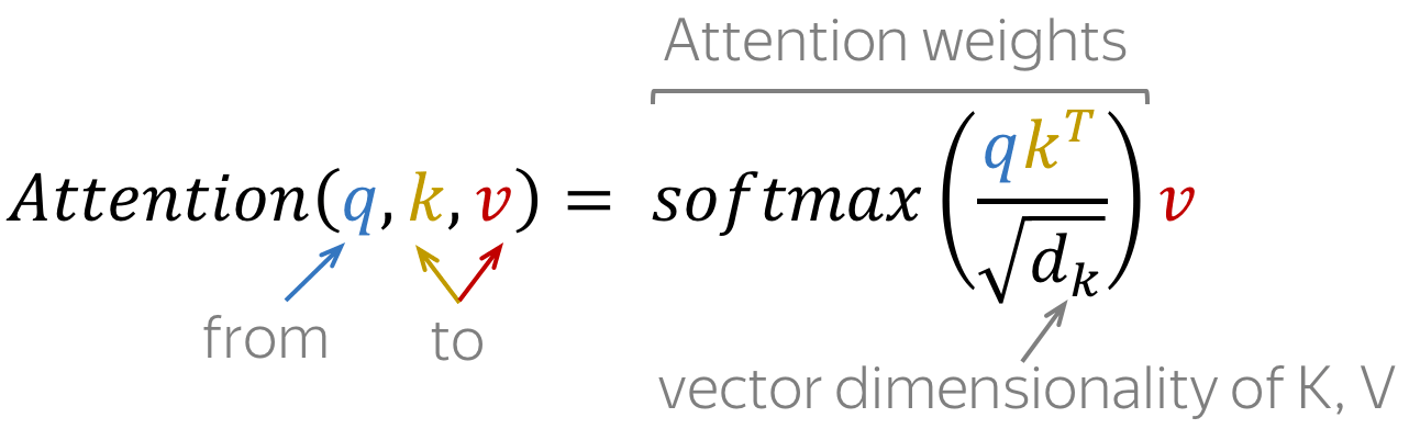
The query is used when a token looks at others - it's seeking the information to understand itself better. The key is responding to a query's request: it is used to compute attention weights. The value is used to compute attention output: it gives information to the tokens which "say" they need it (i.e. assigned large weights to this token).
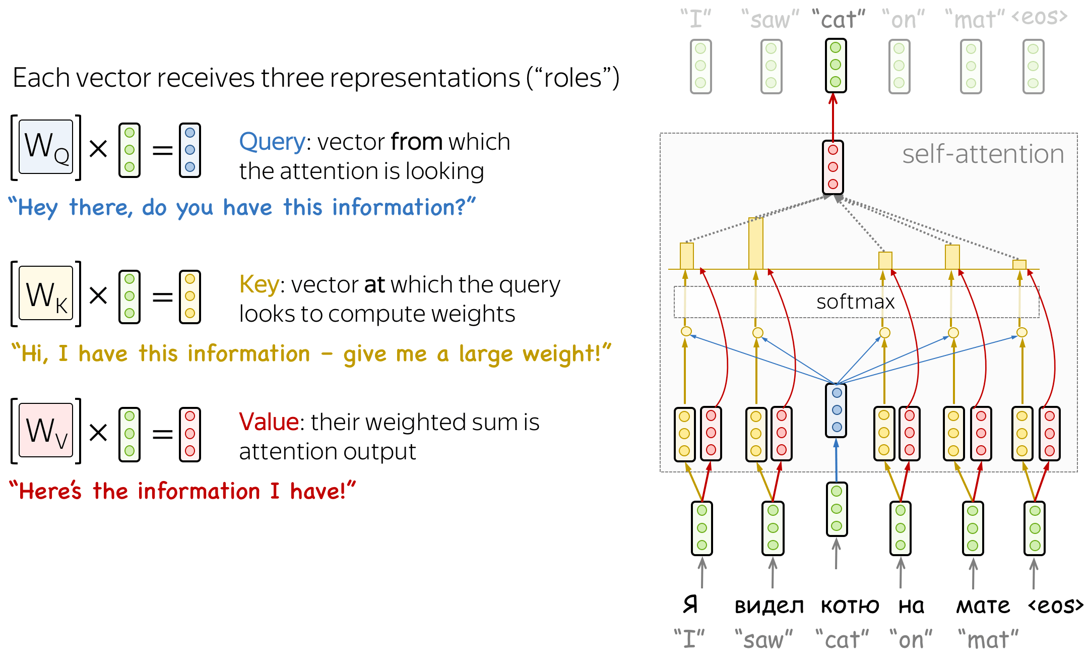
The formula for computing attention output is as follows:
Masked Self-Attention: "Don't Look Ahead" for the Decoder
In the decoder, there's also a self-attention mechanism: it is the one performing the "look at the previous tokens" function.
In the decoder, self-attention is a bit different from the one in the encoder. While the encoder receives all tokens at once and the tokens can look at all tokens in the input sentence, in the decoder, we generate one token at a time: during generation, we don't know which tokens we'll generate in future.
To forbid the decoder to look ahead, the model uses masked self-attention: future tokens are masked out. Look at the illustration.
But how can the decoder look ahead?
During generation, it can't - we don't know what comes next. But in training, we use reference translations (which we know). Therefore, in training, we feed the whole target sentence to the decoder - without masks, the tokens would "see future", and this is not what we want.
This is done for computational efficiency: the Transformer does not have a recurrence, so all tokens can be processed at once. This is one of the reasons it has become so popular for machine translation - it's much faster to train than the once dominant recurrent models. For recurrent models, one training step requires O(len(source) + len(target)) steps, but for Transformer, it's O(1), i.e. constant.
Multi-Head Attention: Independently Focus on Different Things
Usually, understanding the role of a word in a sentence requires understanding how it is related to different parts of the sentence. This is important not only in processing source sentence but also in generating target. For example, in some languages, subjects define verb inflection (e.g., gender agreement), verbs define the case of their objects, and many more. What I'm trying to say is: each word is part of many relations.
Therefore, we have to let the model focus on different things: this is the motivation behind Multi-Head Attention. Instead of having one attention mechanism, multi-head attention has several "heads" which work independently.
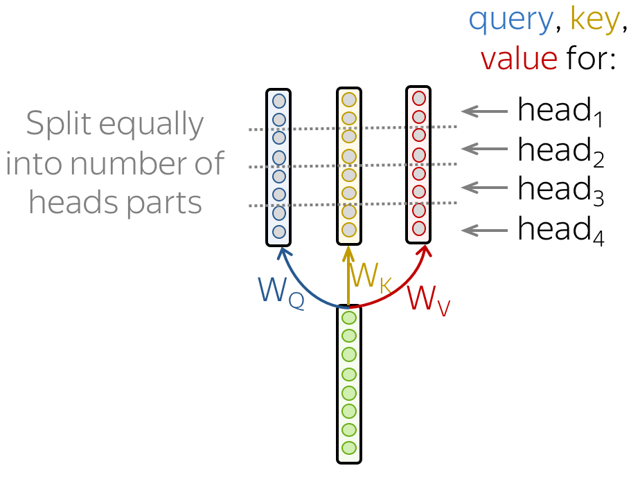
Formally, this is implemented as several attention mechanisms whose results are combined: \[\mbox{MultiHead}(Q, K, V) = \mbox{Concat}(\mbox{head}_1, \dots, \mbox{head}_n)W_o,\] \[\mbox{head}_i=\mbox{Attention}(QW_Q^i, KW_K^i, VW_V^i)\]
In the implementation, you just split the queries, keys, and values you compute for a single-head attention into several parts. In this way, models with one attention head or several of them have the same size - multi-head attention does not increase model size.
In the Analysis and Interpretability section, we will see these heads play different "roles" in the model: e.g., positional or tracking syntactic dependencies.
Transformer: Model Architecture
Now, when we understand the main model components and the general idea, let's look at the whole model. The figure shows the model architecture from the original paper.
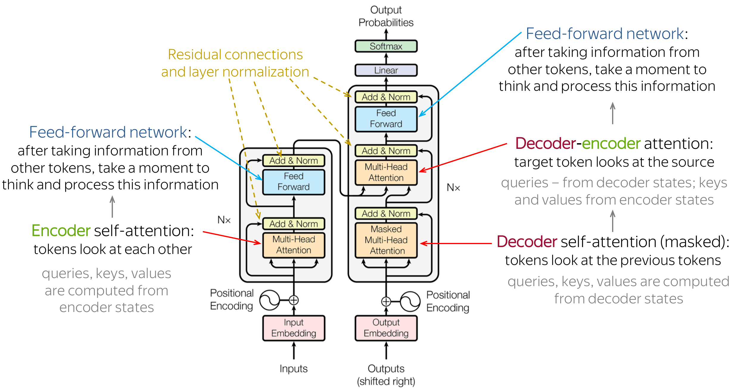
Intuitively, the model does exactly what we discussed before: in the encoder, tokens communicate with each other and update their representations; in the decoder, a target token first looks at previously generated target tokens, then at the source, and finally updates its representation. This happens in several layers, usually 6.
Let's look in more detail at the other model components.
• Feed-forward blocks
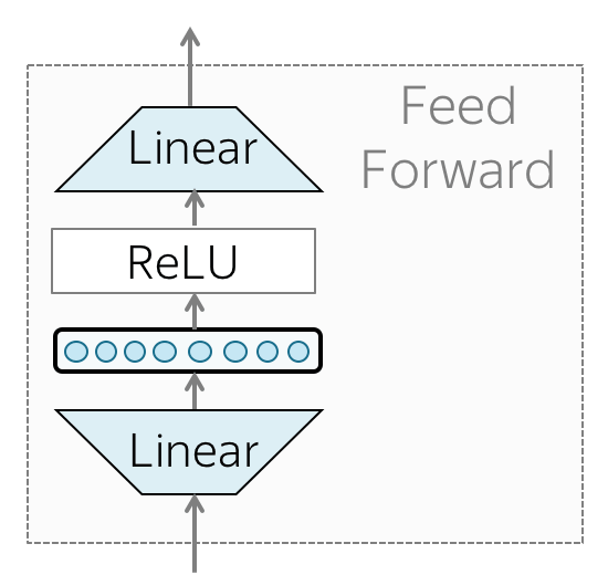
In addition to attention, each layer has a feed-forward network block: two linear layers with ReLU non-linearity between them: \[FFN(x) = \max(0, xW_1+b_1)W_2+b_2.\] After looking at other tokens via an attention mechanism, a model uses an FFN block to process this new information (attention - "look at other tokens and gather information", FFN - "take a moment to think and process this information").
• Residual connections
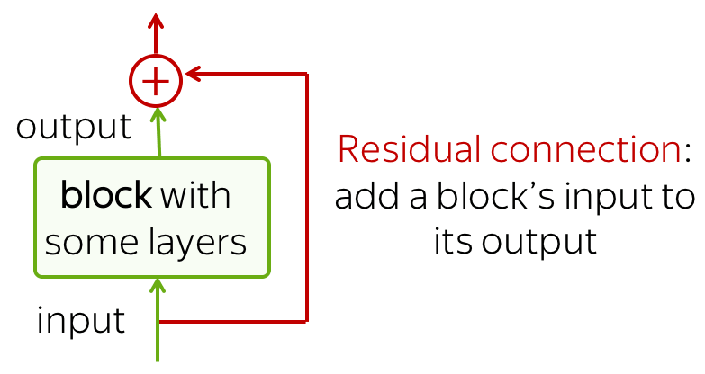
We already saw residual connections when talking about convolutional language models. Residual connections are very simple (add a block's input to its output), but at the same time are very useful: they ease the gradient flow through a network and allow stacking a lot of layers.
In the Transformer, residual connections are used after each attention and FFN block. On the illustration above, residuals are shown as arrows coming around a block to the yellow "Add & Norm" layer. In the "Add & Norm" part, the "Add" part stands for the residual connection.
• Layer Normalization
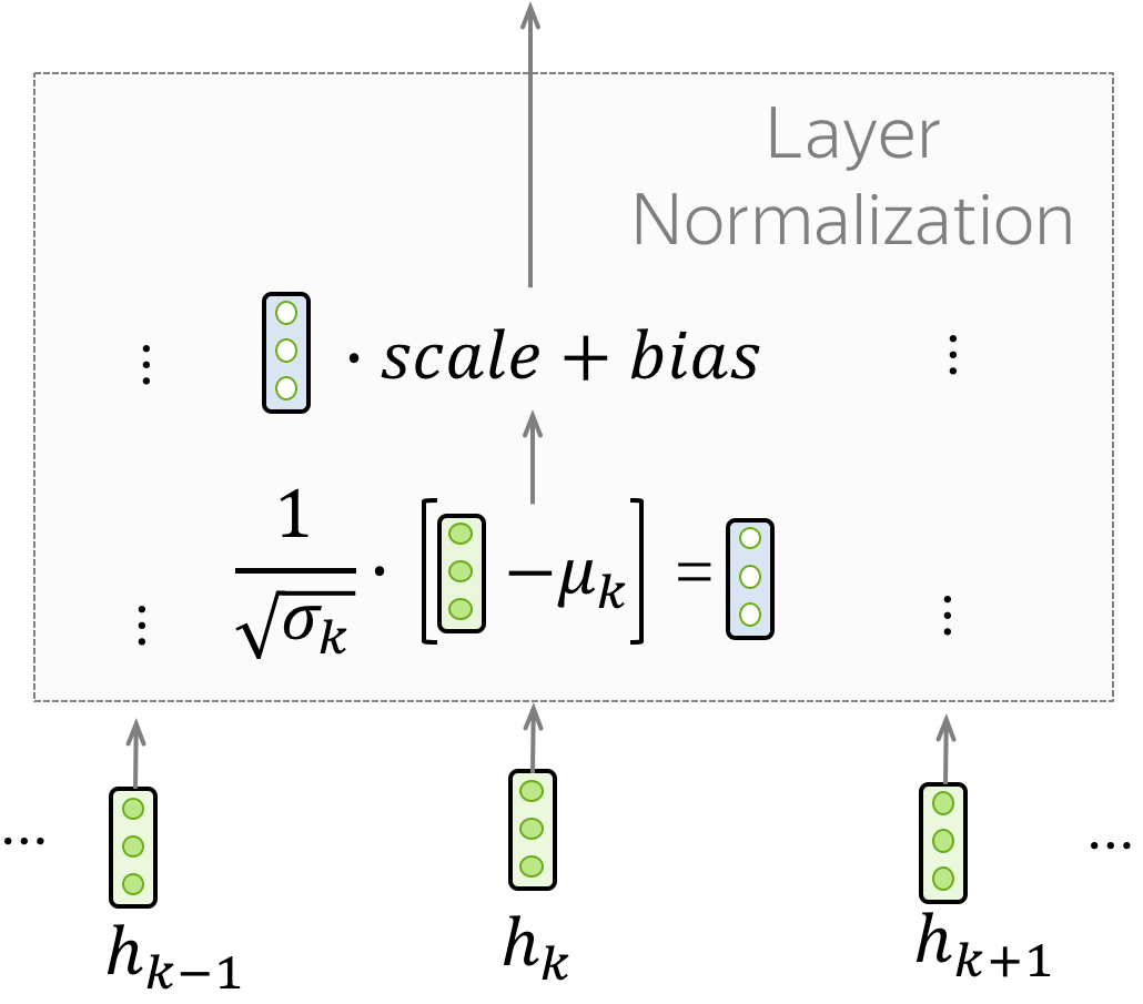
The "Norm" part in the "Add & Norm" layer denotes Layer Normalization. It independently normalizes vector representation of each example in batch - this is done to control "flow" to the next layer. Layer normalization improves convergence stability and sometimes even quality.
In the Transformer, you have to normalize vector representation of each token. Additionally, here LayerNorm has trainable parameters, \(scale\) and \(bias\), which are used after normalization to rescale layer's outputs (or the next layer's inputs). Note that \(\mu_k\) and \(\sigma_k\) are evaluated for each example, but \(scale\) and \(bias\) are the same - these are layer parameters.
• Positional encoding
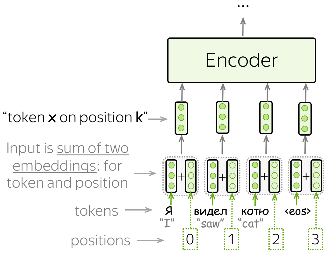
Note that since Transformer does not contain recurrence or convolution, it does not know the order of input tokens. Therefore, we have to let the model know the positions of the tokens explicitly. For this, we have two sets of embeddings: for tokens (as we always do) and for positions (the new ones needed for this model). Then input representation of a token is the sum of two embeddings: token and positional.
The positional embeddings can be learned, but the authors found that having fixed ones does not hurt the quality. The fixed positional encodings used in the Transformer are: \[\mbox{PE}_{pos, 2i}=\sin(pos/10000^{2i/d_{model}}),\] \[\mbox{PE}_{pos, 2i+1}=\cos(pos/10000^{2i/d_{model}}),\] where \(pos\) is position and \(i\) is the vector dimension. Each dimension of the positional encoding corresponds to a sinusoid, and the wavelengths form a geometric progression from 2π to 10000 · 2π.
Subword Segmentation: Byte Pair Encoding
As we know, a model has a predefined vocabulary of tokens. Those input tokens, which are not in the vocabulary, will be replaced with a special UNK ("unknown") token. Therefore, if you use the straightforward word-level tokenization (i.e., your tokens are words), you will be able to process a fixed number of words. This is the fixed vocabulary problem : you will be getting lot's of unknown tokens, and your model won't translate them properly.
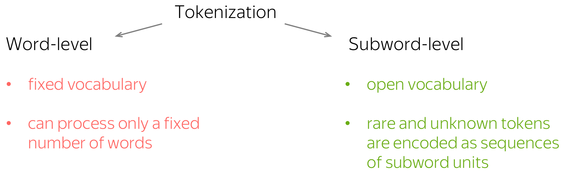
But how can we represent all words, even those we haven't seen in the training data? Well, even if you are not familiar with a word, you are familiar with the parts it consists of - subwords (in the worst case, symbols). Then why don't we split the rare and unknown words into smaller parts?
This is exactly what was proposed in the paper Neural Machine Translation of Rare Words with Subword Units by Rico Sennrich, Barry Haddow and Alexandra Birch. They introduced the de-facto standard subword segmentation, Byte Pair Encoding (BPE). BPE keeps frequent words intact and splits rare and unknown ones into smaller known parts.
How does it work?
The original Byte Pair Encoding (BPE) (Gage, 1994) is a simple data compression technique that iteratively replaces the most frequent pair of bytes in a sequence with a single, unused byte. What we refer to as BPE now is an adaptation of this algorithm for word segmentation. Instead of merging frequent pairs of bytes, it merges characters or character sequences.
BPE algorithm consists of two parts:
- training - learn "BPE rules", i.e., which pairs of symbols to merge;
- inference - apply learned rules to segment a text.
Let's look at each of them in more detail.
Training: learn BPE rules
At this step, the algorithm builds a merge table and a vocabulary of tokens. The initial vocabulary consists of characters and an empty merge table. At this step, each word is segmented as a sequence of characters. After that, the algorithm is as follows:
- count pairs of symbols: how many times each pair occurs together in the training data;
- find the most frequent pair of symbols;
- merge this pair - add a merge to the merge table, and the new token to the vocabulary.
In practice, the algorithm first counts how many times each word appeared in the data. Using this information, it can count pairs of symbols more easily. Note also that the tokens do not cross word boundary - everything happens within words.
Look at the illustration. Here I show you a toy example: here we assume that in training data, we met cat 4 times, mat 5 times and mats, mate, ate, eat 2, 3, 3, 2 times, respectively. We also have to set the maximum number of merges we want; usually, it's going to be about 4k-32k depending on the dataset size, but for our toy example, let's set it to 5.
When we reached the maximum number of merges, not all words were merged into a single token. For example, mats is segmented as two tokens: mat@@ s. Note that after segmentation, we add the special characters @@ to distinguish between tokens that represent entire words and tokens that represent parts of words. In our example, mat and mat@@ are different tokens.
Implementation note. In an implementation, you need to make sure that a new merge adds only one new token to the vocabulary. For this, you can either add a special end-of-word symbol to each word (as done in the original BPE paper) or replace spaces with a special symbol (as done in e.g. Sentencepiece and YouTokenToMe, the fastest implementation), or do something else. In the illustration, I omit this for simplicity.
Inference: segment a text
After learning BPE rules, you have a merge table - now, we will use it to segment a new text.
The algorithm starts with segmenting a word into a sequence of characters. After that, it iteratively makes the following two steps until no merge it possible:
- among all possible merges at this step, find the highest merge in the table;
- apply this merge.
Note that the merge table is ordered - the merges that are higher in the table were more frequent in the data. That's why in the algorithm, merges that are higher have higher priority: at each step, we merge the most frequent merge among all possible.
Note that while BPE segmentation is deterministic,
even with the same vocabulary a word can have different segmentations, e.g.
un relat ed,
u n relate d,
un rel ated,
etc.). Maybe it would be better to use different segmentations in training?
Well, maybe it would. Learn more in this exercise
in the Research Thinking section.
Analysis and Interpretability
Multi-Head Self-Attention: What are these heads doing?
First, let's start with our traditional model analysis method: looking at model components. Previously, we looked at convolutional filters in classifiers, neurons in language models; now, it's time to look at a bigger component: attention. But let's take not the vanilla one, but the heads in Transformer's multi-head attention.
Lena: First, why are we doing this? Multi-head attention is an inductive bias introduced in the Transformer. When creating an inductive bias in a model, we usually have some kind of intuition for why we think this new model component, inductive bias, could be useful. Therefore, it's good to understand how this new thing works - does it learn the things we thought it would? If not, why it helps? If yes, how can we improve it? Hope now you are motivated enough, so let's continue.
The Most Important Heads are Interpretable
Here we'll mention some of the results from the ACL 2019 paper Analyzing Multi-Head Self-Attention: Specialized Heads Do the Heavy Lifting, the Rest Can Be Pruned. The authors look at individual attention heads in encoder's multi-head attention and evaluate how much, on average, different heads "contribute" to generated translations (for the details on how exactly they did this, look in the paper or the blog post). As it turns out,
- only a small number of heads are important for translation,
- these heads play interpretable "roles".
These roles are:
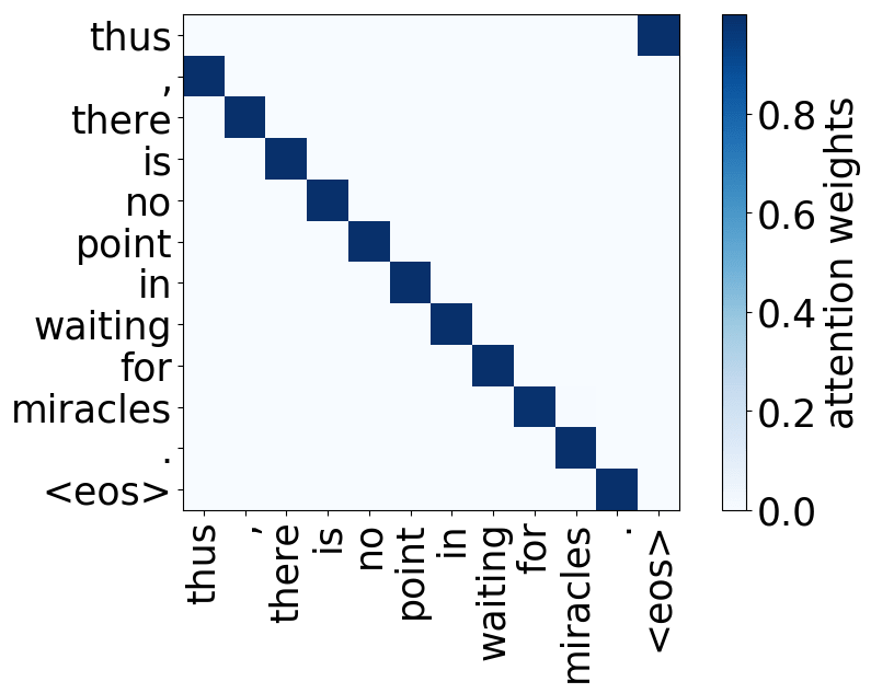
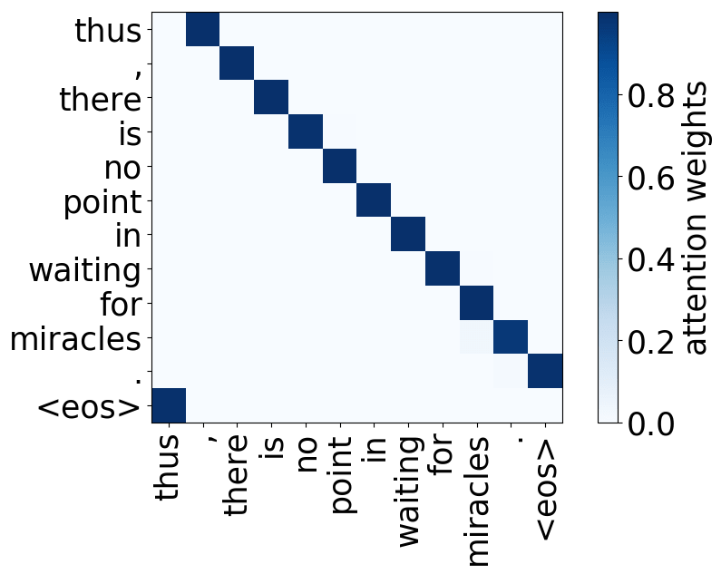
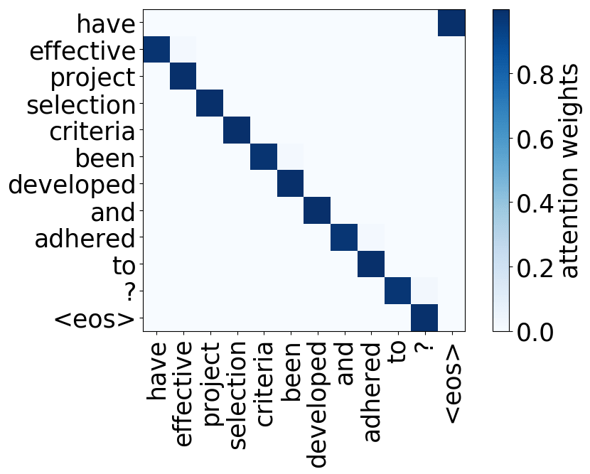
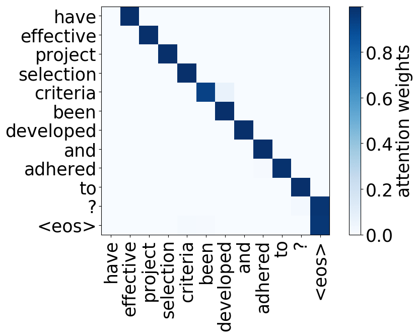
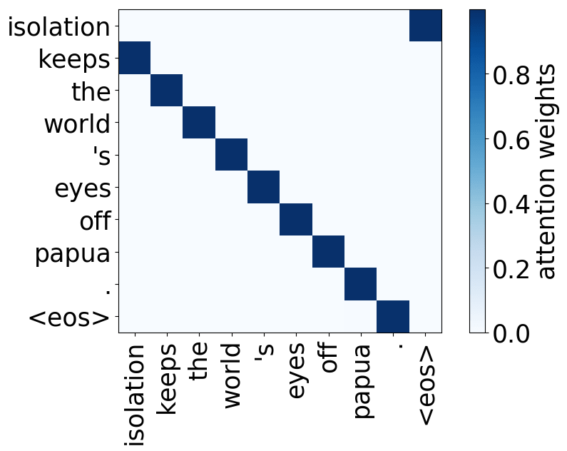
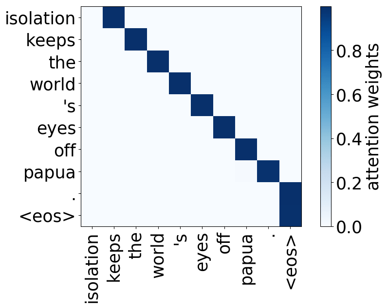
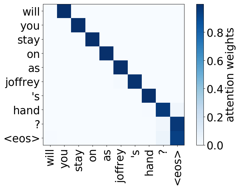
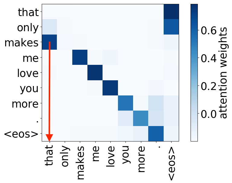
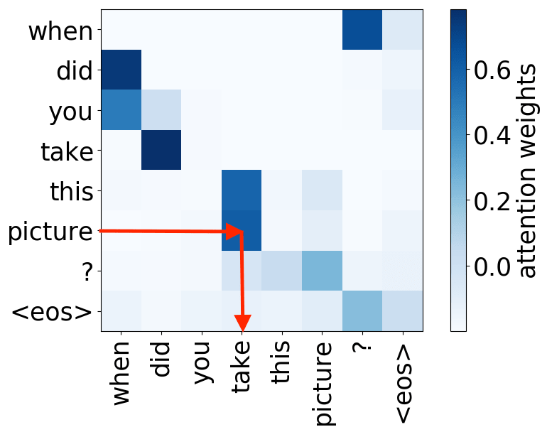
- positional: attend to a token's immediate neighbors, and the model has several such heads (usually 2-3 heads looking at the previous token and 2 heads looking at the next token);
- syntactic: learned to track some major syntactic relations in the sentence (subject-verb, verb-object);
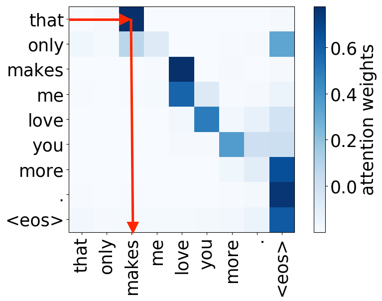
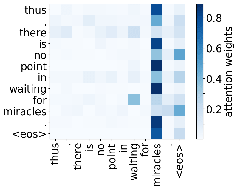
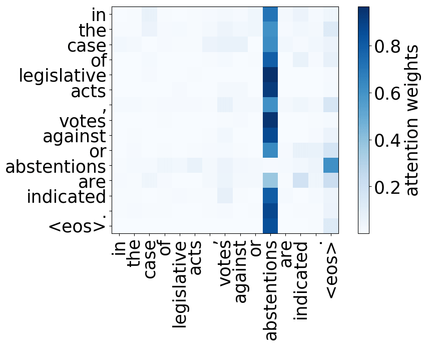
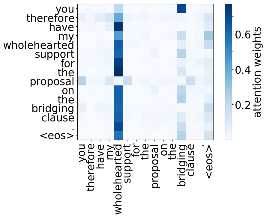
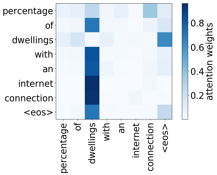
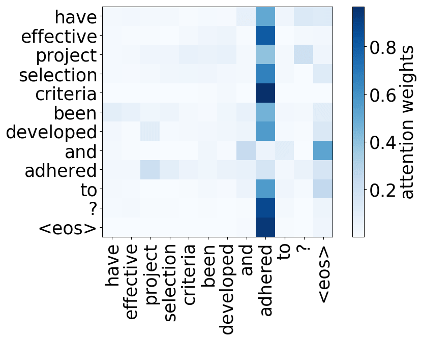
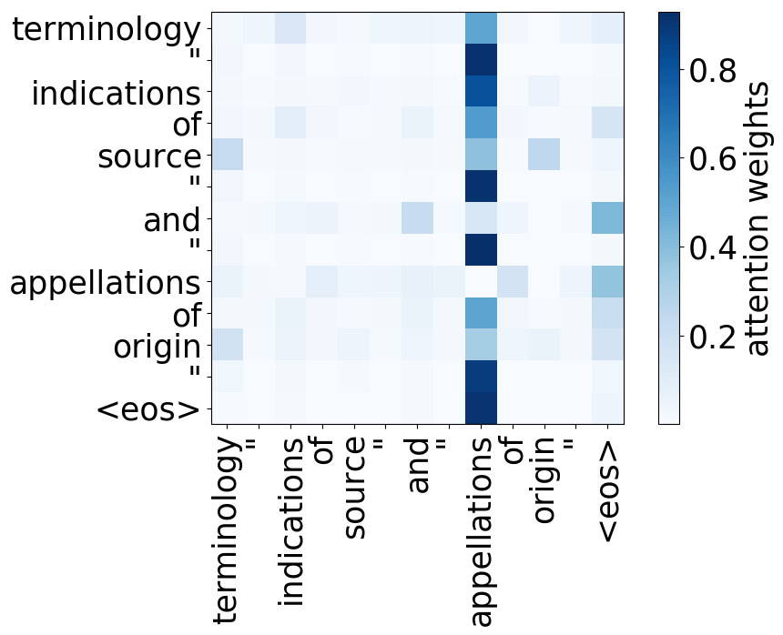
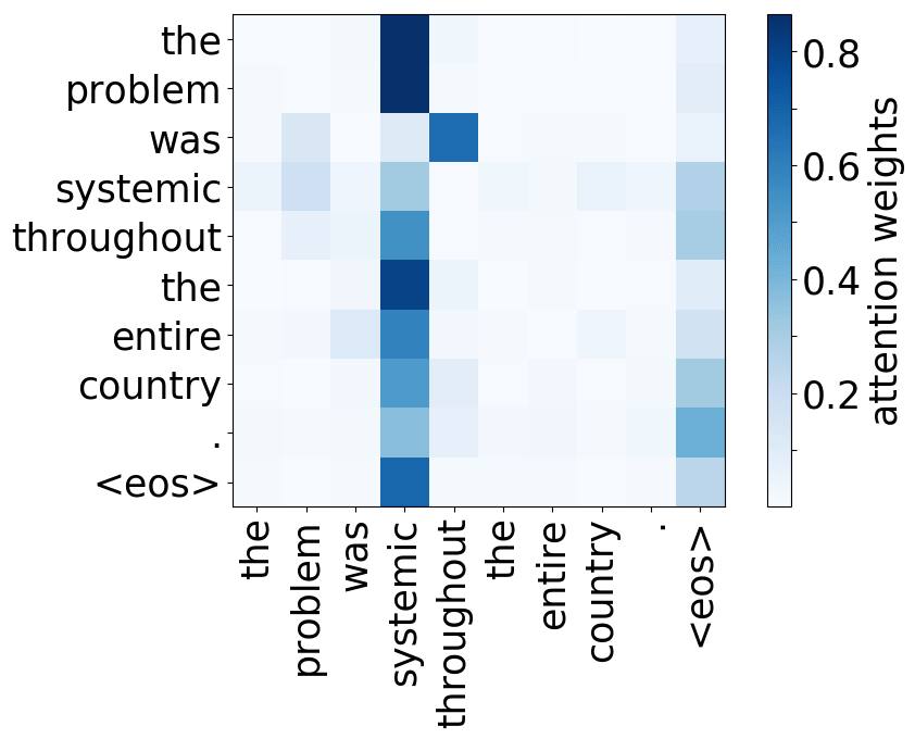
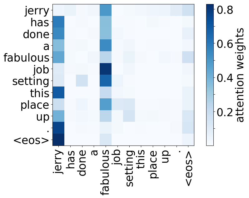
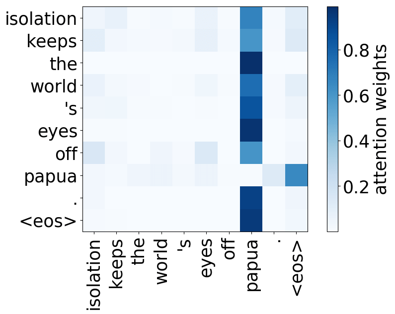
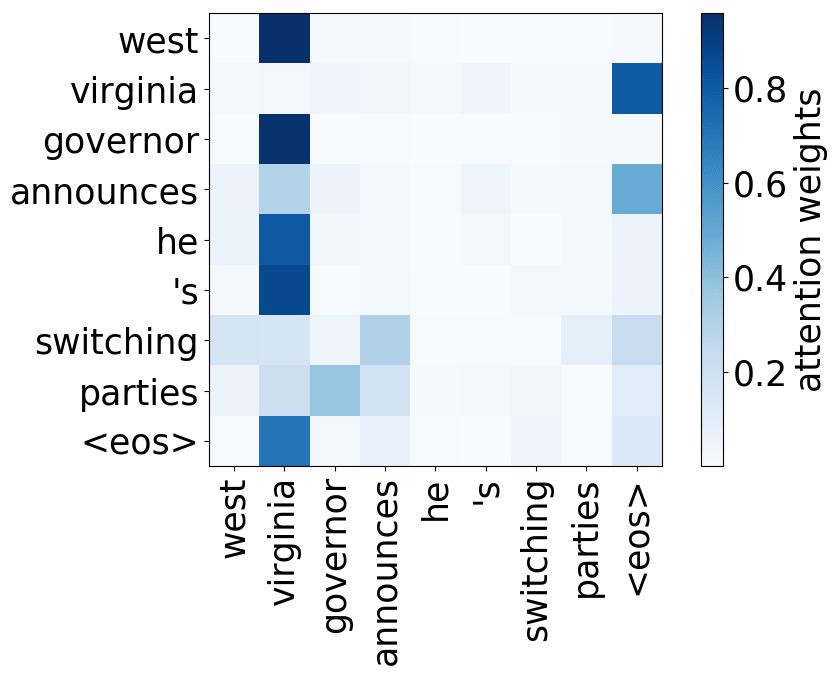
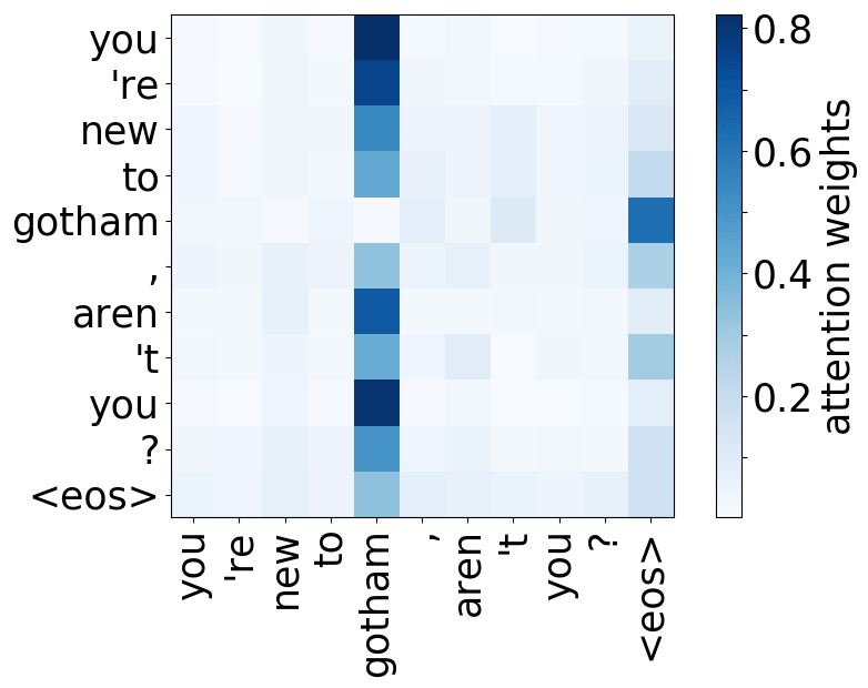
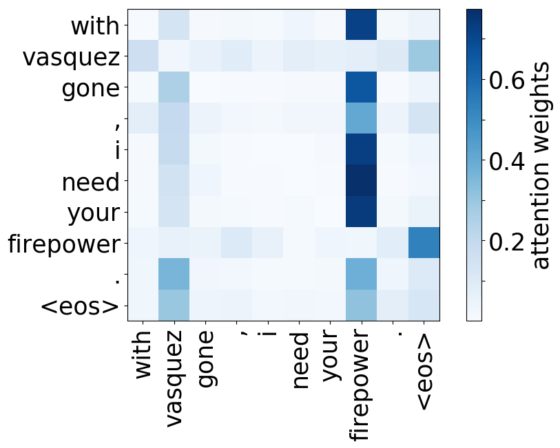
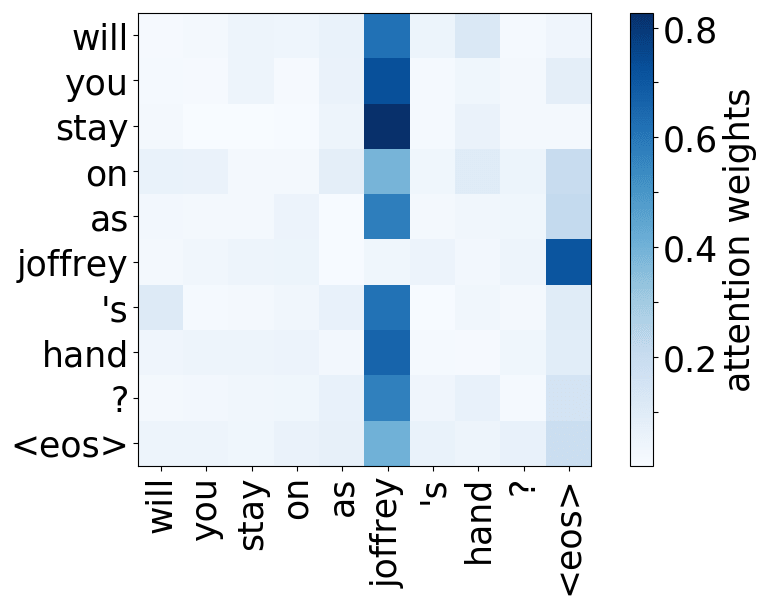
- rare tokens: the most important head on the first layer attends to the least frequent tokens in a sentence (this is true for models trained on different language pairs!).
Look at the examples of positional and syntactic heads below. This means that our intuition for having several heads was right - among other things, the model did learn to track relations between words!
Positional heads
Model trained on WMT EN-DE
Model trained on WMT EN-DE
Model trained on WMT EN-FR
Model trained on WMT EN-FR
Model trained on WMT EN-RU
Model trained on WMT EN-RU
Model trained on OpenSubtitles EN-RU
Model trained on OpenSubtitles EN-RU
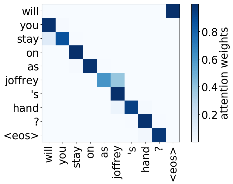
Syntactic heads
subject-> verb
verb -> subject
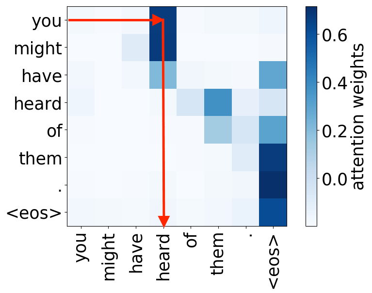
subject-> verb
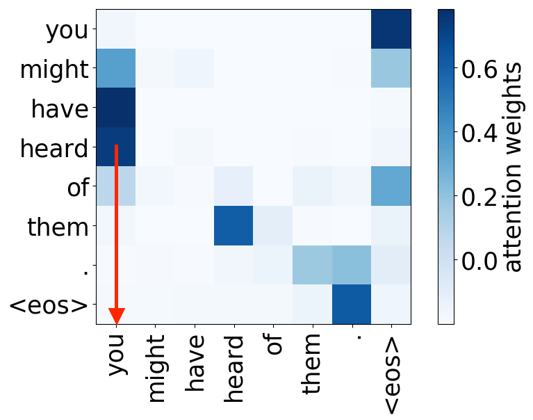
verb -> subject
verb -> subject
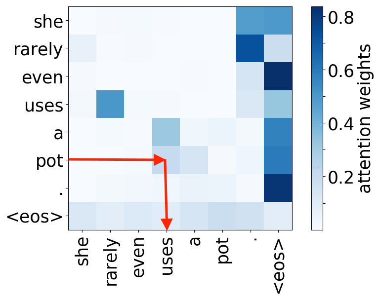
object -> verb
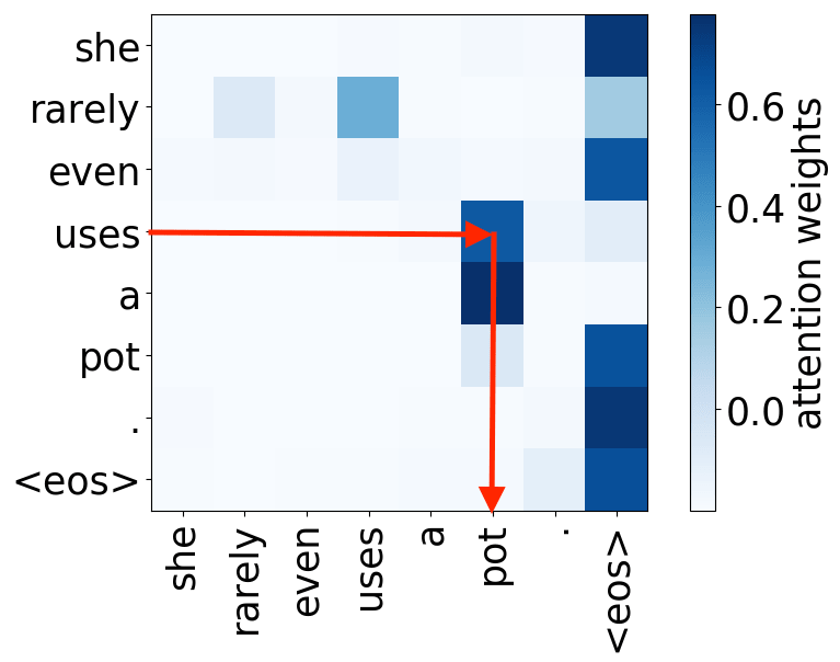
verb -> object
object -> verb
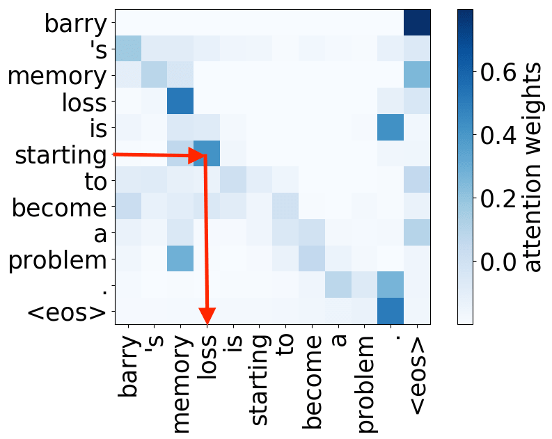
Rare tokens head
Model trained on WMT EN-DE
Model trained on WMT EN-DE
Model trained on WMT EN-DE
Model trained on WMT EN-FR
Model trained on WMT EN-FR
Model trained on WMT EN-FR
Model trained on WMT EN-RU
Model trained on WMT EN-RU
Model trained on WMT EN-RU
Model trained on WMT EN-RU
Model trained on OpenSubtitles EN-RU
Model trained on OpenSubtitles EN-RU
Model trained on OpenSubtitles EN-RU
While the rare tokens head surely looks fun, don't overestimate it - most probably, this is a sign of overfitting. By looking at the least frequent tokens, a model tries to hang on to these rare "clues".
The Majority of the Heads Can be Pruned
Later on in the paper, the authors let the model decide which heads it does not need (again, for more details look in the paper or the blog post) and iteratively prunes attention heads, i.e. removes them from the model. In addition to confirming that the specialized heads are the most important (because the model keeps them intact and prunes the other ones), the authors find that most of the heads can be removed without significant loss in quality.
Why don't we train a model with a small number of heads to begin with?
Well, you can't - the quality will be much lower. You need many heads in training to let them learn all these useful things.
Probing: What Do Representations Capture?
Note that looking at model components is a model-specific approach: the components you may be interested in and ways of "looking" at them depend on the model.
Now we are interested in model-agnostic methods. For example, what do representations in the model learn? Do they learn to encode some linguistic features? Here we will feed the data to a trained network, gather vector representations of this data, and will try to understand whether these vectors encode something interesting.
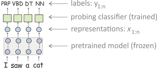
The most popular approach is to use probing classifiers (aka probes, probing tasks, diagnostic classifiers). In this setting, you
- feed data to a network and get vector representations of this data,
- train a classifier to predict some linguistic labels from these representations (but the model itself is frozen and is used only to produce representations),
- use the classifier's accuracy as a measure of how well representations encode labels.
This approach for analysis is (for now) the most popular in NLP, and we will meet it again when talking about transfer learning in the next lecture. Now, let's look at some examples of how it can be used to analyze NMT models.
Lena: Recently, it turned out that the accuracy of a probing classifier is not a good measure, and you need to modify what you evaluate using a probing classifier. But this is a very different story...
What do NMT Models Learn about Morphology?
In this part, let's look at the ACL 2017 paper What do Neural Machine Translation Models Learn about Morphology? The authors trained NMT systems (LSTM ones) on several language pairs and analyzed the representations of these models. Here I will mention only some results to illustrate how you can use probing for analysis.
• Part of Speech Tags
One of the experiments looks at how well encoder representations capture part-of-speech tags (POS tags). For each of the encoder layers starting from embeddings, the authors trained a classifier to predict POS tags from representations from this layer. The results are shown in the figure (layer 0 - embeddings, layer 1 and 2 - encoder layers).
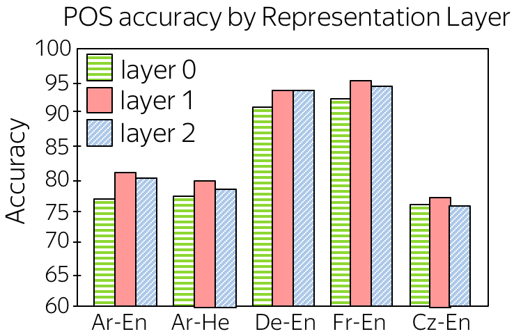
We can see that
- passing embeddings through encoder improves POS tagging
This is expected - while layer 0 knows only current token, representations from encoder layers know its context and can understand part of speech better. - layer 1 is better than layer 2
The hypothesis is that while layer 1 captures word structure, layer 2 encodes more high-level information (e.g., semantic).
• The Effect of Target Language
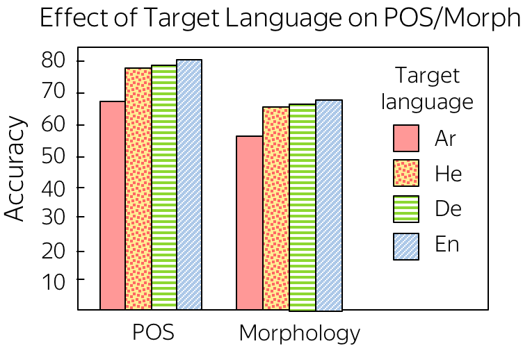
Another interesting question the authors look at the effect of the target language. Given the same source language (Arabic) and different target languages, encoders trained with which target language will learn more about source morphology? For target languages, the authors took Arabic, Hebrew (morphologically-rich language with similar morphology to the source language), German (a morphologically-rich language with different morphology), and English (a morphologically-poor language).
Somewhat unexpectedly, weaker target morphology forces a model to understand source morphology better.
Research Thinking
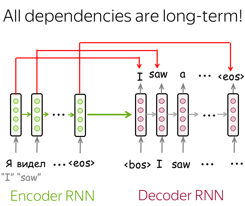
Simple LSTMs without Attention
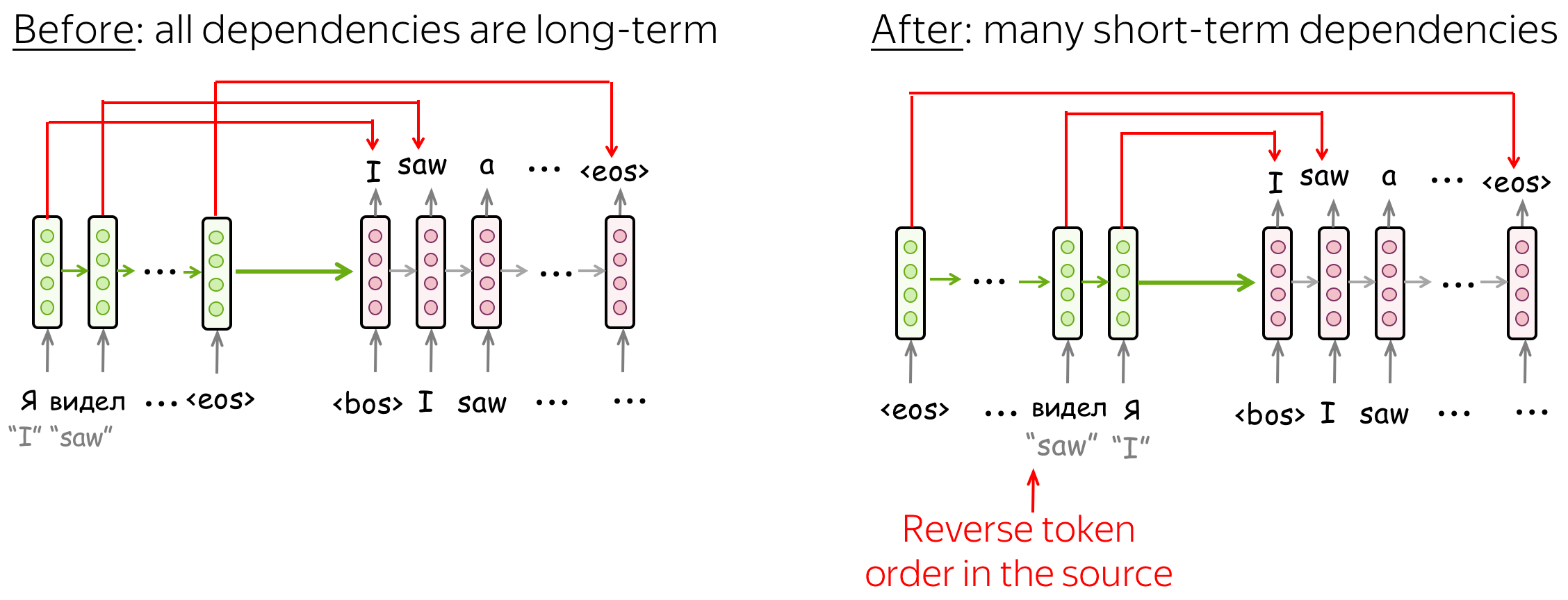
Simple LSTMs without attention does not work very well: all dependencies are long-term, and it is hard for the model. For example, by the time the decoder has to generate the beginning of a translation, it may already forget the most relevant early source tokens.
Possible answers
Reverse order of source tokens
The paper Sequence to Sequence Learning with Neural Networks introduced an elegant trick to make simple LSTM seq2seq models work better: reverse the order of the source tokens (but not the target). After that, a model will have many short-term connections: the latest source tokens it sees are the most relevant for the beginning of the target.
Improve Subword Segmentation
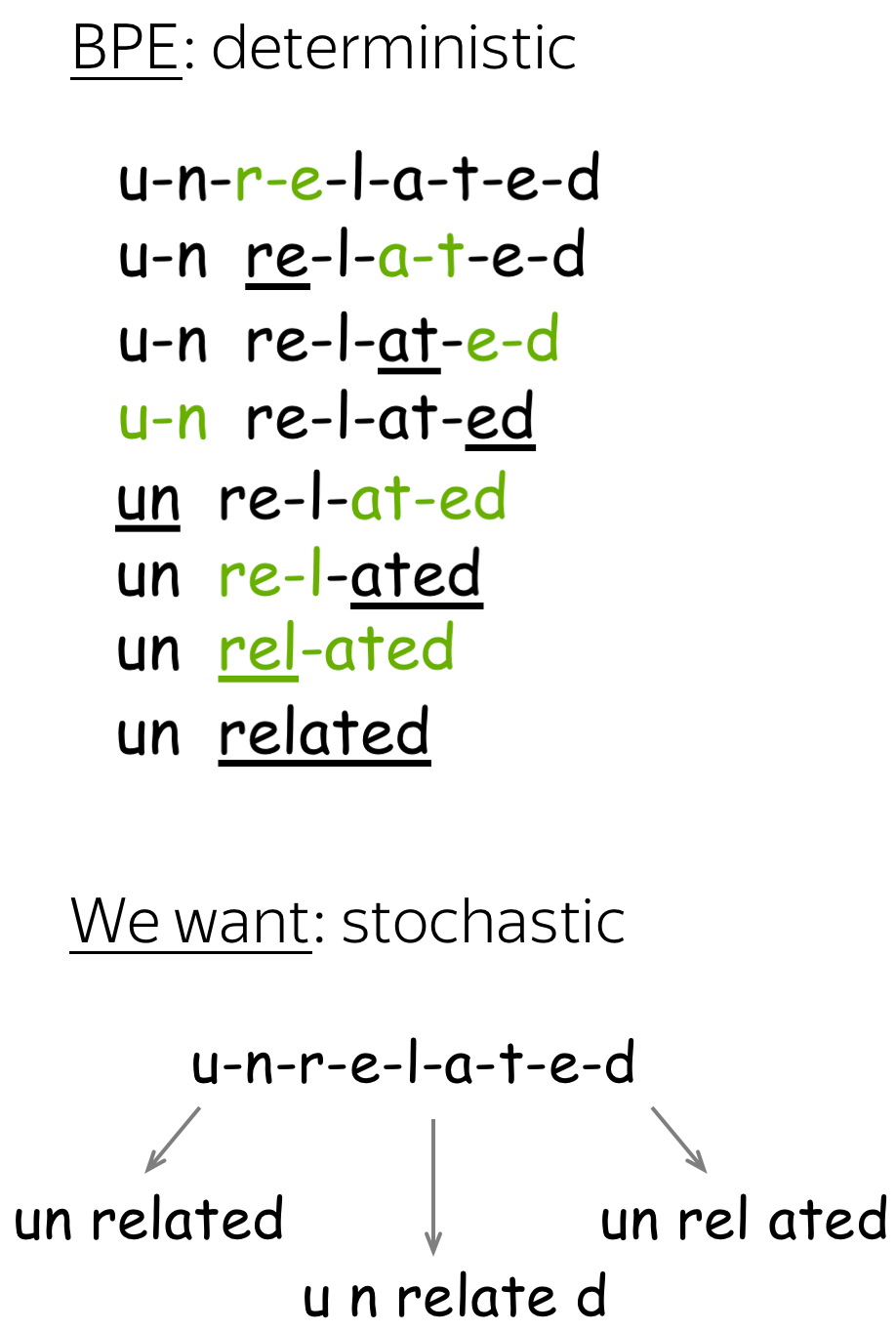
The standard BPE segmentation is deterministic: at each step, it always picks the highest merge in the table. However, even with the same vocabulary, a word can have different segmentations, e.g. un relat ed, u n relate d, un rel ated, etc.).
Imagine that during training of an NMT model each time we pick one of the several possible segmentations - i.e. the same word can be segmented differently. We use the same merge table built by the standard BPE, and the standard segmentation at test time - we modify only training.
Possible answers
Possible reasons why showing different segmentations of the same word can help a model are:
- with different segmentations of a word, a model can better understand the subwords it consists of. Therefore, it can better understand word composition.
- since only rare and unknown words are split into subwords, a model may not learn representations for subwords very well. With different segmentations, it will see subwords in many different contexts and will understand them better.
- this may serve as a regularization - a model will learn not to over-rely on individual tokens and to consider a broader context (similar to the standard word dropout).
To back up these points, let's pick several rare tokens and look at their closest neighbors. To find closest neighbors, we use embeddings from two models trained with (1) BPE and with (2) a stochastic segmentation (which we will look at in the next question).
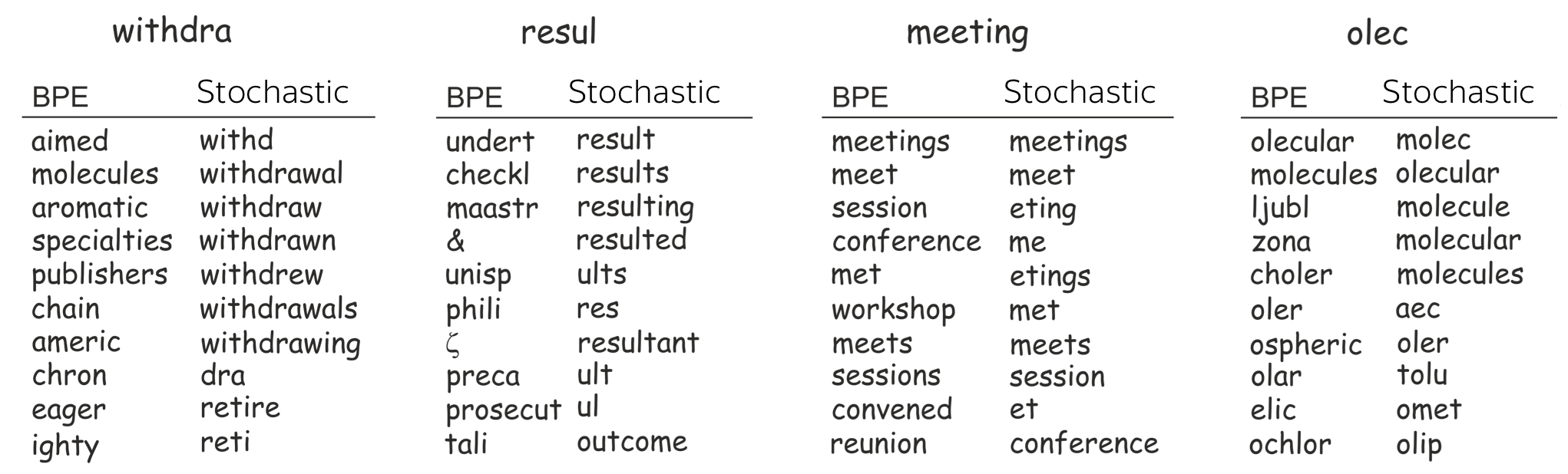
We see that, indeed, a model with stochastic segmentation understands words better. Closest neighbors in the embeddings space of the stochastic segmentation share common parts, which is not the case for BPE.
Note BPE has this problem is only for rare tokens - for frequent ones, the neighbors are reasonable.
Possible answers
BPE-Dropout: drop some merges from the merge table
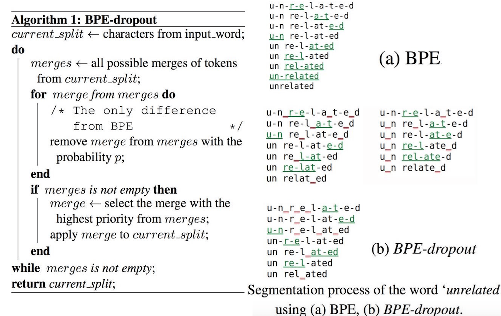
Let's consider BPE-dropout: the approach proposed in the ACL 2020 paper BPE-Dropout: Simple and Effective Subword Regularization.
The idea is very simple: if BPE is deterministic because we pick the highest merge, all we need to do is to (sometimes) pick other merges. For this, the authors randomly drop some merges (e.g., 10% of all merges) from the BPE merge table. In this case, the highest merge is sometimes dropped from the table, we'll have to pick the other one, and the segmentation will be different.
The algorithm and examples of segmentations for the token unrelated is shown below. Red underlines show the merges dropped at each step. Note that the merges to be dropped are chosen at each step again.
In the paper, there're lots of experiments showing improvements in quality from using BPE-dropout as well as the analysis of why this happens. You already saw some part of this analysis in the previous question when looking at the closest neighbors in the embeddings spaces.
Here will be more exercises!
This part will be expanding from time to time.

Related Papers
Here will be papers!
The papers will be gradually appearing.

Have Fun!
Coming soon!
We are still working on this!