Text Classification
Multi-class classification:
many labels, only one correct
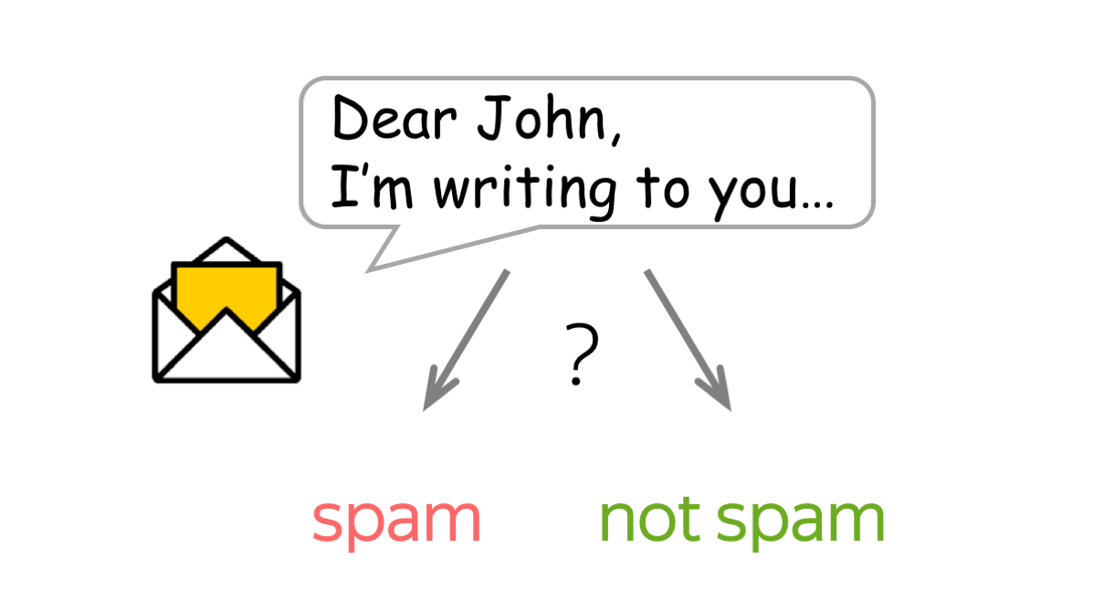
Binary classification:
two labels, only one correct
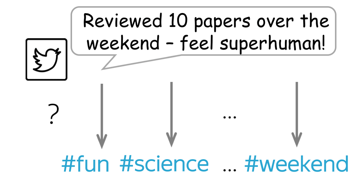
Multi-label classification:
many labels, several can be correct
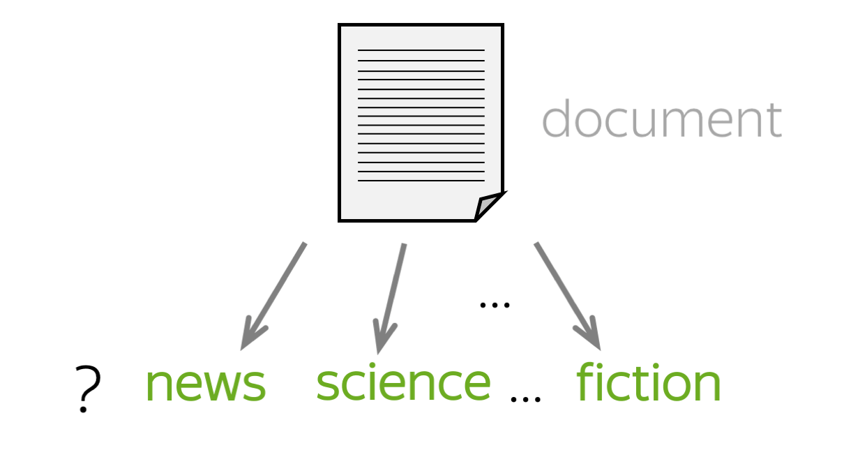
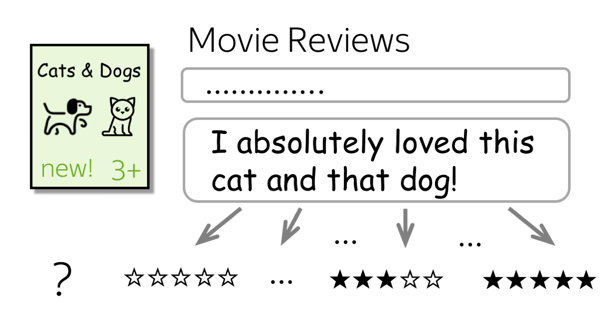
Multi-class classification:
many labels, only one correct
Text classification is an extremely popular task. You enjoy working text classifiers in your mail agent: it classifies letters and filters spam. Other applications include document classification, review classification, etc.
Text classifiers are often used not as an individual task, but as part of bigger pipelines. For example, a voice assistant classifies your utterance to understand what you want (e.g., set the alarm, order a taxi or just chat) and passes your message to different models depending on the classifier's decision. Another example is a web search engine: it can use classifiers to identify the query language, to predict the type of your query (e.g., informational, navigational, transactional), to understand whether you what to see pictures or video in addition to documents, etc.
Since most of the classification datasets assume that only one label is correct (you will see this right now!), in the lecture we deal with this type of classification, i.e. the single-label classification. We mention multi-label classification in a separate section (Multi-Label Classification).
Datasets for Classification
Datasets for text classification are very different in terms of size (both dataset size and examples' size), what is classified, and the number of labels. Look at the statistics below.
| Dataset | Type | Number of labels | Size (train/test) | Avg. length (tokens) |
|---|---|---|---|---|
| SST | sentiment | 5 or 2 | 8.5k / 1.1k | 19 |
| IMDb Review | sentiment | 2 | 25k / 25k | 271 |
| Yelp Review | sentiment | 5 or 2 | 650k / 50k | 179 |
| Amazon Review | sentiment | 5 or 2 | 3m / 650k | 79 |
| TREC | question | 6 | 5.5k / 0.5k | 10 |
| Yahoo! Answers | question | 10 | 1.4m / 60k | 131 |
| AG’s News | topic | 4 | 120k / 7.6k | 44 |
| Sogou News | topic | 6 | 54k / 6k | 737 |
| DBPedia | topic | 14 | 560k / 70k | 67 |
The most popular datasets are for sentiment classification. They consist of reviews of movies, places or restaurants, and products. There are also datasets for question type classification and topic classification.
To better understand typical classification tasks, below you can look at the examples from different datasets.
How to: pick a dataset and look at the examples to get a feeling of the task. Or you can come back to this later!
Dataset Description (click!)
SST is a sentiment classification dataset which consists of movie reviews (from Rotten Tomatoes html files). The dataset consists of parse trees of the sentences, and not only entire sentences, but also smaller phrases have a sentiment label.
There are five labels: 1 (very negative), 2 (negative), 3 (neutral), 4 (positive), and 5 (very positive) (alternatively, labels can be 0-4). Depending on the used labels, you can get either binary SST-2 dataset (if you only consider positivity and negativity) or fine-grained sentiment SST-5 (when using all labels).
Note that the dataset size mentioned above (8.5k/2.2k/1.1k for train/dev/test) is in the number of sentences. However, it also has 215,154 phrases that compose each sentence in the dataset.
For more details, see the original paper.
Look how sentiment of a sentence is composed from its parts.
Label: 3
Review:
Makes even the claustrophobic on-board quarters seem fun .
Label: 1
Review:
Ultimately feels empty and unsatisfying , like swallowing a Communion wafer without the wine .
Label: 5
Review:
A quiet treasure -- a film to be savored .
Dataset Description (click!)
IMDb is a large dataset of informal movie reviews from the Internet Movie Database. The collection allows no more than 30 reviews per movie. The dataset contains an even number of positive and negative reviews, so randomly guessing yields 50% accuracy. The reviews are highly polarized: they are only negative (with the highest score 4 out of 10) or positive (with the lowest score 7 out of 10).
For more details, see the original paper.
Label: negative
Review
Hobgoblins .... Hobgoblins .... where do I begin?!?
This film gives Manos -
The Hands of Fate and Future War a run for their money as the worst film ever made .
This one is fun to laugh at , where as Manos was just painful to watch . Hobgoblins will
end up in a time capsule somewhere as the perfect movie to describe the term : " 80 's cheeze " .
The acting ( and I am using this term loosely ) is atrocious , the Hobgoblins are some of the worst
puppets you will ever see , and the garden tool fight has to be seen to be believed .
The movie was the perfect vehicle for MST3 K , and that version is the only way to watch this mess .
This movie gives Mike and the bots lots of ammunition to pull some of the funniest one -
liners they have ever done . If you try to watch this without the help of Mike and the bots .....
God help you ! !
Label: positive
Review
One of my favorite movies I saw at preview in Seattle . Tom Hulce was amazing , with out words could
convey his feelings / thoughts . I actually sent Mike Ferrell some donation money to help the film
get distributed . It is good . System says I need more lines but do not want to give away plot stuff .
I was in the audience in Seattle with Hulce and director , a writer I think and Mike Ferrell .
They talked for about an hour afterwords . Not really a dry eye in the house . Why Hollywood continues
to be stupid I do not know . ( actually I do know , it is our fault , look what we watch)Well you get
what you pay for guys . Get this and see it with someone special . It is a gem .
Label: negative
Review
Okay , if you have a couple hours to waste , or if you just really hate your life , I would say watch
this movie . If anything it 's good for a few laughs . Not only do you have obese , topless natives ,
but also special effects so bad they are probably outlawed in most states . Seriuosly ,
the rating of ' PG ' is pretty humorous too , once you see the Native Porn Extravaganza .
I would n't give this movie to my retarded nephew . You could n't even show this to Iraqi
prisoners without violating the Geneva Convention . The plot is sketchy , and cliché , and dumb ,
and stupid . The acting is horrible , and the ending is so painful to watch I actually began pouring
salt into my eye just to take my mind off of the idiocy filling my TV screen .
Label: positive
Review
I really liked this movie ... it was cute . I enjoyed it , but if you did n't , that is your fault .
Emma Roberts played a good Nancy Drew , even though she is n't quite like the books . The old fashion
outfits are weird when you see them in modern times , but she looks good on them . To me , the rich
girls did n't have outfits that made them look rich . I mean , it looks like they got all the clothes
-blindfolded- at a garage sale and just decided to put it on all together . All of the outfits
were tacky , especially when they wore the penny loafers with their regular outfits . I do not
want to make the movie look bad , because it definitely was n't ! Just go to the theater and
watch it ! ! ! You will enjoy it !
Label: negative
Review
I always found Betsy Drake rather creepy , and this movie reinforces that . As another review said ,
this is a stalker movie that is n't very funny . I watched it because it has CG in it ,
but he hardly gets any screen time . It 's no " North by Northwest " ...
Label: negative
Review
This movie was on t.v the other day , and I did n't enjoy it at all . The first George of the
jungle was a good comedy , but the sequel .... completely awful . The new actor and
actress to play the lead roles were n't good at all , they should of had the original
actor ( Brendon Fraiser ) and original actress ( i forgot her name ) so this movie gets
the 0 out of ten rating , not a film that you can sit down and watch and enjoy ,
this is a film that you turn to another channel or take it back to the shop if hired or
bought . It was good to see Ape the ape back , but was n't as fun as the first ,
they should of had the new George as Georges son grown up , and still had Bredon and
( what s her face ) in the film , that would 've been a bit better then it was .
Label: positive
Review
I loved This Movie . When I saw it on Febuary 3rd I knew I had to buy It ! ! ! It comes out to buy
on July 24th ! ! ! It has cool deaths scenes , Hot girls , great cast , good story , good
acting . Great Slasher Film . the Movies is about some serial killer killing off four girls .
SEE this movies
Label: positive
Review
gone in 60 seconds is a very good action comedy film that made over $ 100 million but got blasted
by most critics . I personally thought this was a great film . The story was believable and
has probobly the greatest cast ever for this type of movie including 3 academy award winners
nicolas cage , robert duvall and the very hot anjolina jolie . other than the lame stunt
at the end this is a perfect blend of action comedy and drama .
my score is * * * * ( out of * * * * )
Label: positive
Review
This is one of the most interesting movies I have ever seen . I love the backwoods feel of this movie .
The movie is very realistic and believable . This seems to take place in another era , maybe
the late 60 's or early 70 's . Henry Thomas works well with the young baby . Very moving story
and worth a look .
Label: positive
Review
I admit it 's very silly , but I 've practically memorized the damn thing ! It holds a lot of good
childhood memories for me ( my brother and I saw it opening day ) and I have respect for
any movie with FNM on the soundtrack .
Label: positive
Review
I love the series ! Many of the stereotypes portraying Southerrners as hicks are very apparent ,
but such people do exist all too frequently . The portrayal of Southern government rings
all too true as well , but the sympathetic characters reminds one of the many good things
about the South as well . Some things never change , and we see the " good old boys " every day !
There is a Lucas Buck in every Southern town who has only to make a phone call to make things
happen , and the storybook " po ' white trash " are all too familiar . Aside from the supernatural
elements , everything else could very well happen in the modern South ! I somehow think Trinity ,
SC must have been in Barnwell County !
Dataset Description (click!)
The Yelp reviews dataset is obtained from the Yelp Dataset Challenge in 2015. Depending on the number of labels, you can get either Yelp Full (all 5 labels) or Yelp Polarity (positive and negative classes) dataset. Full has 130,000 training samples and 10,000 testing samples in each star, and the Polarity dataset has 280,000 training samples and 19,000 test samples in each polarity.
For more details, see the Kaggle Challenge page.
Label: 4
Review
I had a serious craving for Roti. So glad I found this place.
A very small menu selection but it had exactly what I wanted. The serving for
$8.20 after tax is enough for 2 meals. I know where to go from now on for a great
meal with leftovers. This is a noteworthy place to bring my Uncle T.J. who's a Trini
when he comes to visit.
Label: 2
Review
The actual restaurant is fine, the service is friendly and good.
I am not going to go in to the food other than to say, no.
Oh well $340 bucks and all I can muster is a no.
Label: 5
Review
What a cool little place tucked away behind a strip mall. Would never have found
this if it was not suggested by a good friend who raved about the cappuccino!
He is world traveler, so, it's a must try if it's the best cup he's ever had.
He was right! Don't know if it's in the beans or the care that they take to make
it with a fab froth decoration on top. My hubby and I loved the caramel brulee taste..
My son loved the hot ""warm"" cocoa. Yeah, we walked in as a family last night and
almost everyone turned our way since we did not fit the hip college crowd.
Everyone was really friendly, though. The sweet young man behind the
counter gave my son some micro cinnamon doughnuts and scored major points with the
little dude! We will be back.
Label: 3
Review
Jersey Mike's is okay. It's a chain place, and a bit over priced for fast food.
I ordered a philly cheese steak. It was mostly bread, with a few
thing microscopic slices of meat. A little cheese too. And a sliver or
two of peppers. But mostly, it was bread. I think it's funny the people
that work here try to make small talk with you. "So, what are you guys up to tonight?"
I think it would be fun to just try and f*#k with them, and say something like,
"Oh you know, smoking a little meth and just chilling with some hookers."
See what they say to that.
Label: 5
Review
Love it!!! Wish we still lived in Arizona as Chino is the one thing we miss.
Every time I think about Chino Bandido my mouth starts watering.
If I am ever in the state again I will drive out of my way just to go to it again. YUMMY!
Label: 4
Review
I have been here a few times, but mainly at dinner. Dinner Has always been great, great
waiters and staff, with a LCD TV playing almost famous famous bolywood movies.
LOL It cracks me up when they dance.....LOL...anyhow, Great vegetarian choices for
people who eat there veggies, but trust me, I am a MEAT eater, Chicekn Tika masala,
Little dry but still good. My favorite is there Palak Paneer. Great for the vegetarian.
I have also tried there lunch Buffet for 11.00. I give a Thumbs up.. Good,
serve yourself, and pig out!!!!!!
Label: 3
Review
Very VERY average. Actually disappointed in the braciole. Kelsey with the pretty smile and form
fitting shorts would probably make me think about going back and trying something different.
Label: 1
Review
So, what kind of place serves chicken fingers and NO Ranch dressing?????? The only sauces they
had was honey mustard and ""Canes Secret sauce"" Can I say EEWWWW!! I thought that
the sauce tasted terrible. I am not too big a fan of honey mustard but I do On occasion
eat it if there is nothing else And that wasn't even good! The coleslaw was awful also.
I do have to say that the chicken fingers were very juicy but also very bland.
Those were the only 2 items that I tried, not that there were really any more items on
the menu, Texas toast? And Fries I think?? Overall, I would never go back.
Label: 4
Review
Good food, good drinks, fun bar.
There are quite a few Buffalo Wild Wings in the valley and they're a fun place to grab a quick lunch or dinner and watch the game.
They have a pretty good garden burger and their buffalo chips (french fry-ish things) are really good.
If you like bloody mary's, they have the best one. It's so good...really spicy and filled with celery and olives.
Be careful when you come though, if there is a game on, you'll have to get there early or you definitely won't get a spot to sit.
Label: 5
Review
Excellent in every way. Attentive and fun owners who tend bar every weekend night - GREAT live music,
excellent wine selection. Keeping Fountain Hills young.... one weekend at a time.
Label: 1
Review
After repeat visits it just gets worse - the service, that is. It was as if we were held
hostage and could not leave for a full 25 minutes because that's how long it took to receive
hour check after several requests to several different employees. Female servers might
be somewhat cute but know absolutely nothing about beer and this is a brewpub.
I asked if they have an seasonal beers and the reply was no, that they only sell
their own beers! Even more amusing is their ""industrial pale ale"" is an IPA but it
is not bitter. So, they say it's an IPA but it's not bitter, it's not a true-to-style IPA.
Then people say ""Oh I don't like IPA's"" and want something else. Their attempt
to rename a beer/style is actually hurting them. Amazing.
Dataset Description (click!)
The Amazon reviews dataset consists of reviews from amazon which include product and user information, ratings, and a plaintext review. The dataset is obtained from the Stanford Network Analysis Project (SNAP). Depending on the number of labels, you can get either Amazon Full (all 5 labels) or Amazon Polarity (positive and negative classes) dataset. Full has 600,000 training samples and 130,000 testing samples in each star, and the Polarity dataset has 1800,000 training samples and 200,000 test samples in each polarity. The fields used are review title and review content.
Label: 4
Review Title: good for a young reader
Review Content:
just got this book since i read it when i was younger and loved it. i will reread it one
of these days, but i bet its pretty lame 15 years later, oh well.
Label: 2
Review Title: The Castle in the Attic
Review Content:
i read the castle in the attic and i thoght it wasn't very entrtaning.
but that's just my opinion. i thought on some of the chapters it dragged
on and lost me alot. like it would talk about one thing and then another without
alot of detail. for my opinion, it was an ok book. it had it's moments like whats
going to happen next then it was really boring.
Label: 1
Review Title: worst book in the world!!!!!!!!!!!!!!!!!!!!!!!!!!!!!!!!!!!!
Review Content:
This was the worst book I have ever read in my entire life! I was forced to read it for
school. It was complicated and very boring. I would not recommend this book to anyone!!
Please don't waste your time and money to read this book!! Read something else!!
Label: 3
Review Title: It's okay.
Review Content:
I'm using it for track at school as a sprinter. It's okay, but to hold it together
is a velcro strap. So you either use the laces or take them out and use only the velcro.
Also, if you order them, order them a half size or a full size biggerthen your normal
size or else it'll be a tight squeeze. Plus side, you can still run on your toes in them.
Label: 5
Review Title: Time Well Spent
Review Content:
For those beginning to read the classics this one is a great hook. While the characters are
complex the story is linear and the allusions are simple enough to follow. One can't help
but hope Tess's life will somehow turn out right although knowing it will not. The burdens
she encounters seem to do little to stop her from moving forward. Life seems so unfair
to her, but Hardy handles her masterfully; indeed it is safe to say Hardy loves her more
than God does.
Label: 2
Review Title: Not a brilliant book but...
Review Content:
I didn't like this book very much. It was silly. I'm sorry that I've wasted time reading
this book. There are better books to read.
Label: 3
Review Title: Simple
Review Content:
This book was not anything special. Although I love romances, it was too simple.
The symbolism was spelled out to the readers in a blunt manner. The less educated
readers may appreciate it. The wording was quite beautiful at times and the plot was
enchanting (perfect for a movie) but it is not heart wrenching like the movie Titantic
(which was a must see!) ;)
Label: 1
Review Title: WHY???????????????????????????????????????????????????
Review Content:
WHY are poor, innocent school kids forced to read this intensly dull text? It is
enough to put anyone off English Lit for LIFE. If anyone in authority is reading
this, PLEASE take this piece of junk OFF the sylabus...PLEASE!!!!!!!!!!!
Label: 4
Review Title: looking back
Review Content:
I have read several Thomas Hardy novels starting with The Mayor of Casterbridge many years
ago in high school and I never really appreciated the style and the fact that like other Hardy
novels Tess is a love story and a very good story. Worth reading
Label: 5
Review Title: Great Puzzle
Review Content:
This is an excellent puzzle for very young children. Melissa & Doug products are well made and kids
love them. This puzzle is wooden so kids wont destroy it if they try to roughly put the pieces in.
The design is adorable and makes a great gift for any young animal lover.
Dataset Description (click!)
TREC is a dataset for classification of free factual questions. It defines a two-layered taxonomy, which represents a natural semantic classification for typical answers in the TREC task. The hierarchy contains 6 coarse classes (ABBREVIATION, ENTITY, DESCRIPTION, HUMAN, LOCATION and NUMERIC VALUE) and 50 fine classes.
For more details, see the original paper.
Label: DESC (description)
Question: How did serfdom develop in and then leave Russia ?
Label: ENTY (entity)
Question: What films featured the character Popeye Doyle ?
Label: HUM (human)
Question: What team did baseball 's St. Louis Browns become ?
Label: HUM (human)
Question: What is the oldest profession ?
Label: DESC (description)
Question: How can I find a list of celebrities ' real names ?
Label: ENTY (entity)
Question: What fowl grabs the spotlight after the Chinese Year of the Monkey ?
Label: ABBR (abbreviation)
Question: What is the full form of .com ?
Label: ENTY (entity)
Question: What 's the second - most - used vowel in English ?
Label: DESC (description)
Question: What are liver enzymes ?
Label: HUM (human)
Question: Name the scar-faced bounty hunter of The Old West .
Label: NUM (numeric value)
Question: When was Ozzy Osbourne born ?
Label: DESC (description)
Question: Why do heavier objects travel downhill faster ?
Label: HUM (human)
Question: Who was The Pride of the Yankees ?
Label: HUM (human)
Question: Who killed Gandhi ?
Label: LOC (location)
Question: What sprawling U.S. state boasts the most airports ?
Label: DESC (description)
Question: What did the only repealed amendment to the U.S. Constitution deal with ?
Label: NUM (numeric value)
Question: How many Jews were executed in concentration camps during WWII ?
Label: DESC (description)
Question: What is " Nine Inch Nails " ?
Label: DESC (description)
Question: What is an annotated bibliography ?
Label: NUM (numeric value)
Question: What is the date of Boxing Day ?
Label: ENTY (entity)
Question: What articles of clothing are tokens in Monopoly ?
Label: HUM (human)
Question: Name 11 famous martyrs .
Label: DESC (description)
Question: What 's the Olympic motto ?
Label: NUM (numeric value)
Question: What is the origin of the name ` Scarlett ' ?
Dataset Description (click!)
The dataset is gathered from Yahoo! Answers Comprehensive Questions and Answers version 1.0 dataset. In contains the 10 largest main categories: "Society & Culture", "Science & Mathematics", "Health, "Education & Reference", "Computers & Internet", "Sports", "Business & Finance", "Entertainment & Music", "Family & Relationships", "Politics & Government". Each class contains 140,000 training samples and 5,000 testing samples. The data consists of question title and content, as well as the best answer.
Label: Society & Culture
Question Title: Why do people have the bird, turkey for thanksgiving?
Question Content: Why this bird? Any Significance?
Best Answer
It is believed that the pilgrims and indians shared wild turkey and venison on the
original Thanksgiving.
Turkey's "Americanness" was established by
Benjamin Franklin, who had advocated for the turkey, not the bald eagle,
becoming the national bird.
Label: Science & Mathematics
Question Title: What is an "imaginary number"?
Question Content: What is an "imaginary number",
and how is it treated in algebra equations?
Best Answer
Imaginary numbers are numbers than when squared equal a negative number, as in i^2 = -1,
where i is the imaginary number. You'll also often see them represented as i = √-1
(that's the square root of -1).
Don't be confused by the poorly chosen name -
imaginary numbers do indeed exist and are used in advanced math, such as in the
physics of electromagnetic fields. The analogy that Wikipedia uses is a good one -
just like you don't need the concept of fractions to count stones, it doesn't mean that
fractions don't exist. :)
Label: Health
Question Title: Does echinacea really help prevent colds?
Question Content: Or is a waste of money...
Best Answer
Well, there appears to be some controvery about this. While some people swear by the
stuff, others say that it has no real effect on overcoming a cold.
Here are some
links, one of which is from a National Institute of Health study. I hope these help
you decide whether to head to the health store or not.
Label: Education & Reference
Question Title: How do I find an out of print book?
Question Content: When I was a kid I remember seeing a book that was like an
yearbook of all newspapers published by the Times during WW II.
Each of the years is compiled into a different book. It gave one a very
uniqie perspecitev into the UK druing the war, and even had advertisements
from thaat time. Anybody out there know how to track such books?
Best Answer
here are several websites that you can find rare or out of print books.
A couple would be alibris.com or abebooks.com. These sites list books by
booksellers all over the country and some internationally.
Label: Computers & Internet
Question Title: How can I record audio directly from the browser to the web server?
Question Content: For a podcasting application, I'd like my web server
to be able to receive audio straight from the browser. Something like a "Push to talk"
button. It seems it's possible to do this with Flash. Is there any other way?
With
Flash, do I need to buy a Macromedia server licence, or are there alternatives to have
Flash on the browser talk to my server?
Best Answer
Userplane has an audio/video recorder that will do that -
you can check it out at http://www.userplane.com/apps/videoRecorder.cfm
Label: Sports
Question Title: Why doesn't the NBA implement a minor leagues?
Question Content: I don't want to see any more High School kids on the court,
shooting airballs and missing defensive assignments.
Best Answer
The NBA does have minor leagues - they're called the CBA, and the International leagues. :)
Seriously - because viewers seem to value explosiveness over efficiency,
I think we're seeing a major shift in the average age of NBA players towards
young athletes that are quicker, high-flying and more resilient to injury.
I wouldn't be surprised at all if by the end of this decade the average age of the
league allstars is well under 25.
Label: Business & Finance
Question Title: When will Google buy Yahoo?
Question Content: The two businesses are very complementary in terms
of strengths and weaknesses. Do we want to beat ourselves up competing with
each other for resources and market share, or unite to beat MSFT?
Best Answer
Their respective market caps are too close for this to ever happen.
Interestingly,
many reporters, analysts and tech pundits that I talk to think that the supposed
competition between Google and Yahoo is fallacious, and that they are very different
companies with very different strategies. Google's true competitor is often seen as
being Microsoft, not Yahoo. This would support your claim that they are complementary.
Label: Entertainment & Music
Question Title: Can someone tell me what happened in Buffy's series finale?
Question Content: I had to work and missed the ending.
Best Answer
The gang makes an attack on the First's army, aided by Willow, who performs a powerful
spell to imbue all of the Potentials with Slayer powers. Meanwhile, wearing the amulet
that Angel brought, Spike becomes the decisive factor in the victory, and Sunnydale is
eradicated. Buffy and the gang look back on what's left of Sunnydale, deciding what
to do next...
--but more importantly, there will no longer be any slaying in Sunnydale,
or is that Sunnyvale....
Label: Family & Relationships
Question Title: How do you know if you're in love?
Question Content: Is it possible to know for sure?
Best Answer
In my experience you just know. It's a long term feeling of always wanting to share
each new experience with the other person in order to make them happy, to laugh or
to know what they think about it. It's jonesing to call even though you just got off
an hour long phone call with them. It's knowing that being with them makes you a
better person. It's all of the above and much more.
Label: Politics & Government
Question Title: How come it seems like Lottery winners are always the
ones that buy tickets in low income areas.?
Question Content: Pure luck or Government's way of trying to balance the rich and the poor.
Best Answer
I would put it down to psychology. People who feel they are well-off feel no need to participate in the
lottery programs. While those who feel they are less than well off think "Why not bet a buck or two
on the chance to make a few million?". It would seem to make sense to me.
addition: Yes Matt -
agreed. I just didn't state it as eloquently. Feeling 'no need to participate' is as you say related to
education, and those well off tend to have a better education.
Dataset Description (click!)
The AG’s corpus was obtained from news articles on the web. From these articles, only the AG’s corpus contains only the title and description fields from the the 4 largest classes.
The dataset was introduced in this paper.
Label: Sci/Tech
Title: Learning to write with classroom blogs
Description
Last spring Marisa Dudiak took her second-grade class in Frederick County,
Maryland, on a field trip to an American Indian farm.
Label: Sports
Title: Schumacher Triumphs as Ferrari Seals Formula One Title
Description
BUDAPEST (Reuters) - Michael Schumacher cruised to a record 12th win of the season in the Hungarian
Grand Prix on Sunday to hand his Ferrari team a sixth successive constructors' title.
Label: Business
Title: DoCoMo and Motorola talk phones
Description
Japanese mobile phone company DoCoMo is in talks to buy 3G handsets from Motorola,
the world's second largest handset maker.
Label: World
Title: Sharon 'backs settlement homes'
Description
Reports say Israeli PM Ariel Sharon has given the green light to new homes in West Bank settlements.
Label: Business
Title: Why Hugo Chavez Won a Landslide Victory
Description
When the rule of Venezuelan President Hugo Chavez was reaffirmed in a landslide 58-42 percent
victory on Sunday, the opposition who put the recall vote on the ballot was stunned.
They obviously don't spend much time in the nation's poor neighborhoods.
Label: Sci/Tech
Title: Free-Speech for Online Gambling Ads Sought
Description
The operator of a gambling news site on the Internet has asked a federal judge to declare that
advertisements in U.S. media for foreign online casinos and sports betting outlets
are protected by free-speech rights.
Label: World
Title: Kerry takes legal action against Vietnam critics (AFP)
Description
AFP - Democratic White House hopeful John Kerry's campaign formally alleged that a group attacking
his Vietnam war record had illegal ties to US President George W. Bush's reelection bid.
Label: Sports
Title: O'Leary: I won't quit
Description
The Villa manager was said to be ready to leave the midlands club unless his assistants
Roy Aitken and Steve McGregor were also given new three-and-a-half year deals.
Label: World
Title: Egypt eyes possible return of ambassador to Israel
Description
CAIRO - Egypt raised the possibility Tuesday of returning an ambassador to Israel soon, according
to the official Mena news agency, a move that would signal a revival of full diplomatic ties
after a four-year break.
Label: Sports
Title: Henry wants silverware
Description
Arsenal striker Thierry Henry insisted there must be an end product to the Gunners'
record-breaking run. As Arsenal equalled Nottingham Forest's 42-game unbeaten League
run Henry said: "Even on the pitch we didn't realise what we had done."
Label: Sci/Tech
Title: Scientists Focus on Algae in Maine Lake (AP)
Description
AP - Scientists would kill possibly thousands of white perch under a project to help restore
the ecological balance of East Pond in the Belgrade chain of lakes in central Maine.
Dataset Description (click!)
The Sogou News corpus
was obtained from the combination of the
SogouCA and SogouCS news corpora.
The dataset consists of news articles (title and content fields) labeled with 5 categories:
“sports”, “finance”, “entertainment”, “automobile” and “technology”.
The original dataset is in Chinese, but you can produce Pinyin – a
phonetic romanization of Chinese.
You can do it using
pypinyin
package combined with jieba
Chinese segmentation system (this is what
the paper introducing the dataset did, and this is what I show you in the examples).
The models for English can then be applied to this dataset without change.
The dataset was introduced in this paper, the dataset in Pinyin can be downloaded here.
Lena: Here I picked very small texts - usually, the samples are much longer.
Label: automobile
Title: tu2 we2n -LG be1i be3n sa4i di4 2 lu2n zha4n ba4
cha2ng ha4o ko3ng jie2 de3ng qi2 sho3u fu4 pa2n ta3o lu4n
Content
xi1n la4ng ti3 yu4 xu4n be3i ji1ng shi2 jia1n 5 yue4 28 ri4 ,LG be1i shi4 jie4 qi2 wa2ng sa4i
be3n sa4i di4 2 lu2n za4i ha2n guo2 ka1i zha4n . zho1ng guo2 qi2 sho3u cha2ng ha4o ,
gu3 li4 , wa2ng ya2o , shi2 yue4 ca1n jia1 bi3 sa4i .
tu2 we2i xia4n cha3ng shu4n jia1n .
wa3ng ye4
bu4 zhi1 chi2 Flash
Label: automobile
Title: qi4 che1 pi2n da4o
Content
xi1n we2n jia3n suo3 :
ke4 la2i si1 le4 300C
go4ng 20 zha1ng
ke3 shi3 jia4n pa2n ca1o zuo4 [ fa1ng xia4ng jia4n l: sha4ng yi1 zha1ng ;
fa1ng xia4ng jia4n r: xia4 yi1 zha1ng ; hui2 che1 : zha1 ka4n yua2n da4 tu2 ]\
ge1ng duo1 tu2 pia4n :
ce4 hua4 : bia1n ji2 : me3i bia1n : zhi4 zuo4 :GOODA ji4 shu4 :
Label: finance
Title: shi2 da2 qi1 huo4 : hua2ng ji1n za3o pi2ng (06-11)
Content
shi4 cha3ng jia1 da4 me3i guo2 she1ng xi1 yu4 qi1 , me3i yua2n ji4n qi1 zo3u shi4 ba3o
chi2 de2 xia1ng da1ng pi2ng we3n , ji1n jia4 ga1o we4i mi2ng xia3n sho4u ya1 ,
xia4 jia4ng to1ng da4o ba3o chi2 wa2n ha3o , zhe4n da4ng si1 lu4 ca1o zuo4 .
gua1n wa4ng
wa3ng ye4
bu4 zhi1 chi2 Flash
hua2ng ji1n qi1 huo4 zi1 xu4n la2n mu4
Dataset Description (click!)
DBpedia is a crow-sourced community effort to extract structured information from Wikipedia. The DBpedia ontology classification dataset is constructed by picking 14 non-overlapping classes from DBpedia 2014. From each of the 14 ontology classes, the dataset contains 40,000 randomly chosen training samples and 5,000 testing samples. Therefore, the total size of the training dataset is 560,000, the testing dataset - 70,000.
The dataset was introduced in this paper.
Label: Company
Title: Marvell Software Solutions Israel
Abstract
Marvell Software Solutions Israel known as RADLAN Computer Communications
Limited before 2007 is a wholly owned subsidiary of Marvell Technology Group that
specializes in local area network (LAN) technologies.
Label: EducationalInstitution
Title: Adarsh English Boarding School
Abstract
Adarsh English Boarding School is coeducational boarding school in Phulbari a suburb
of Pokhara Nepal. Nabaraj Thapa is the founder and chairman of the school. The School
motto reads Education For Better Citizen.
Label: Artist
Title: Esfandiar Monfaredzadeh
Abstract
Esfandiar Monfaredzadeh (Persian : اسفندیار منفردزاده) is an Iranian composer and director.
He was born in 1941 in Tehran His major works are Gheisar Dash Akol Tangna Gavaznha. He has
2 daughters Bibinaz Monfaredzadeh and Sanam Monfaredzadeh Woods (by marriage).
Label: Athlete
Title: Elena Yakovishina
Abstract
Elena Yakovishina (born September 17 1992 in Petropavlovsk-Kamchatsky Russia) is
an alpine skier from Russia. She competed for Russia at the 2014 Winter Olympics
in the alpine skiing events.
Label: OfficeHolder
Title: Jack Masters
Abstract
John Gerald (Jack) Masters (born September 27 1931) is a former Canadian politician.
He served as mayor of the city of Thunder Bay Ontario and as a federal Member of Parliament.
Label: MeanOfTransportation
Title: HMS E35
Abstract
HMS E35 was a British E class submarine built by John Brown Clydebank.
She was laid down on 20 May 1916 and was commissioned on 14 July 1917.
Label: Building
Title: Aspira
Abstract
Aspira is a 400 feet (122 m) tall skyscraper in the Denny Triangle neighborhood
of Seattle Washington. It has 37 floors and mostly consists of apartments.
Construction began in 2007 and was completed in late 2009.
Label: NaturalPlace
Title: Sierra de Alcaraz
Abstract
The Sierra de Alcaraz is a mountain range of the Cordillera Prebética located in Albacete
Province southeast Spain. Its highest peak is the Pico Almenara with an altitude of 1796 m.
Label: Village
Title: Piskarki
Abstract
Piskarki [pisˈkarki] is a village in the administrative district of Gmina Jeżewo
within Świecie County Kuyavian-Pomeranian Voivodeship in north-central Poland.
The village has a population of 135.
Label: Animal
Title: Lesser small-toothed rat
Abstract
The Lesser Small-toothed Rat or Western Small-Toothed Rat (Macruromys elegans) is a
species of rodent in the family Muridae. It is found only in West Papua Indonesia.
Label: Plant
Title: Vangueriopsis gossweileri
Abstract
Vangueriopsis gossweileri is a species of flowering plants in the family Rubiaceae.
It occurs in West-Central Tropical Africa (Cabinda Province Equatorial Guinea and Gabon).
Label: Album
Title: Dreamland Manor
Abstract
Dreamland Manor is the debut album of German power metal band Savage Circus.
The album sounds similar to older classic Blind Guardian.
Label: Film
Title: The Case of the Lucky Legs
Abstract
The Case of the Lucky Legs is a 1935 mystery film the third in a series of Perry
Mason films starring Warren William as the famed lawyer.
Label: WrittenWork
Title: Everybody Loves a Good Drought
Abstract
Everybody Loves a Good Drought is a book written by P. Sainath about his research findings of
poverty in the rural districts of India. The book won him the Magsaysay Award.
General View
Here we provide a general view on classification and introduce the notation. This section applies to both classical and neural approaches.
We assume that we have a collection of documents with ground-truth labels. The input of a classifier is a document \(x=(x_1, \dots, x_n)\) with tokens \((x_1, \dots, x_n)\), the output is a label \(y\in 1\dots k\). Usually, a classifier estimates probability distribution over classes, and we want the probability of the correct class to be the highest.
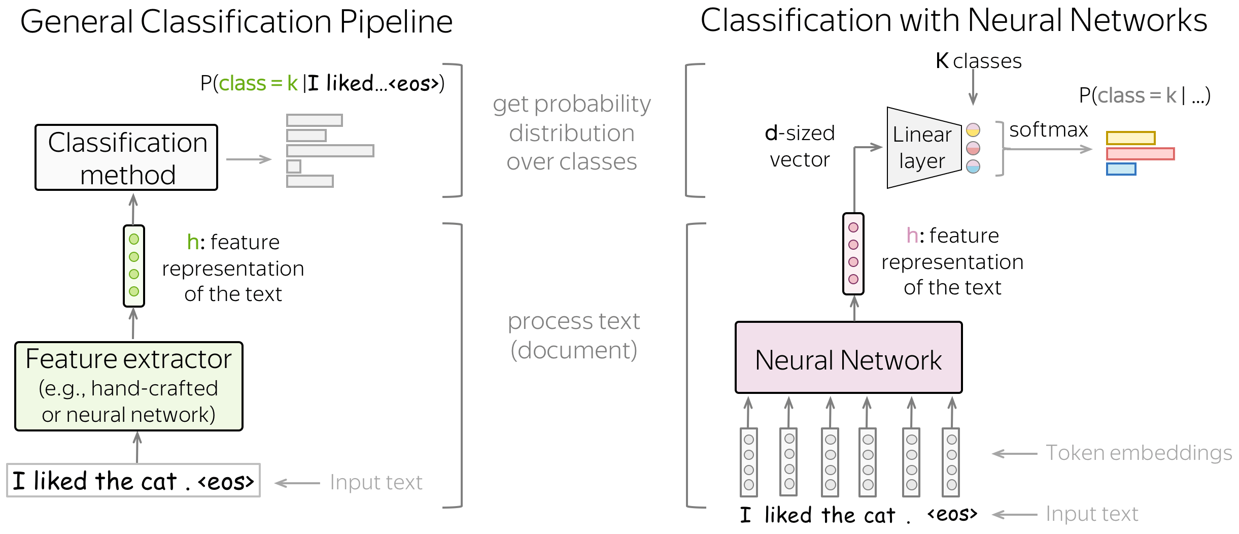
Get Feature Representation and Classify
Text classifiers have the following structure:
- feature extractor
A feature extractor can be either manually defined (as in classical approaches) or learned (e.g., with neural networks). - classifier
A classifier has to assign class probabilities given feature representation of a text. The most common way to do this is using logistic regression, but other variants are also possible (e.g., Naive Bayes classifier or SVM).
In this lecture, we'll mostly be looking at different ways to build feature representation of a text and to use this representation to get class probabilities.
Generative and Discriminative Models
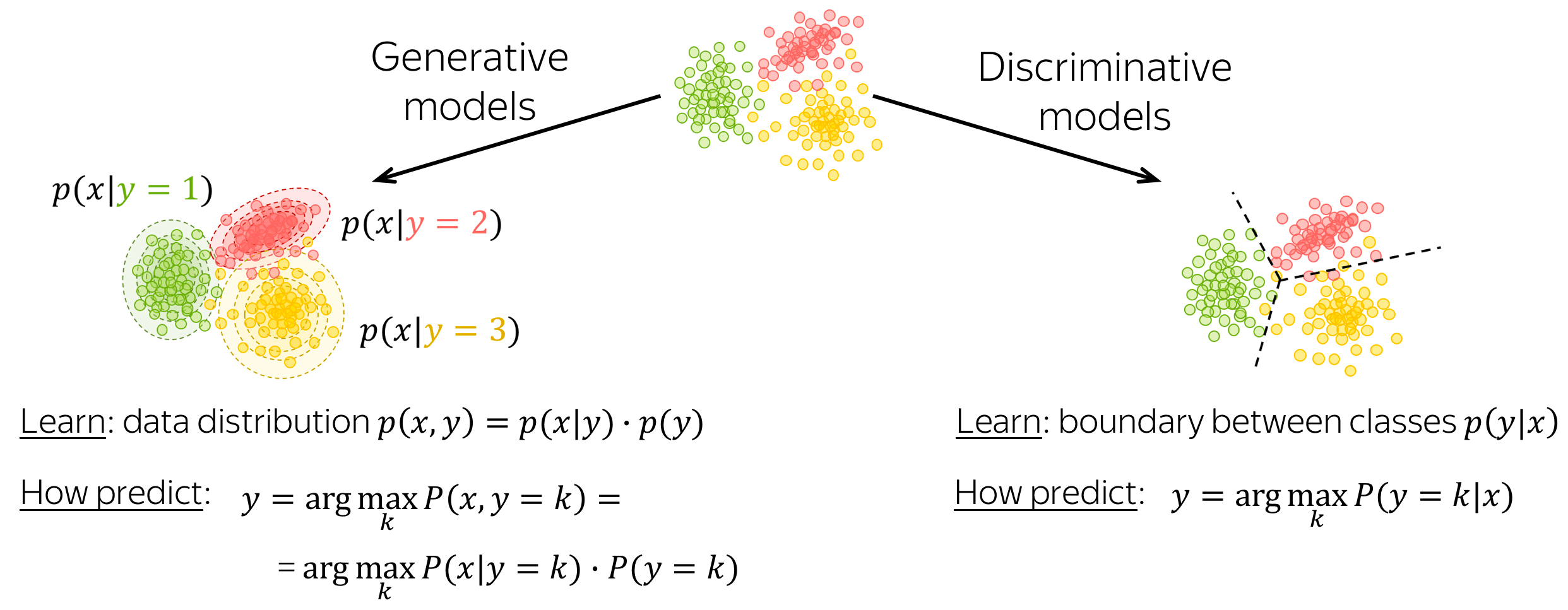
A classification model can be either generative or discriminative.
- generative models
Generative models learn joint probability distribution of data \(p(x, y) = p(x|y)\cdot p(y)\). To make a prediction given an input \(x\), these models pick a class with the highest joint probability: \(y = \arg \max\limits_{k}p(x|y=k)\cdot p(y=k)\). - discriminative models
Discriminative models are interested only in the conditional probability \(p(y|x)\), i.e. they learn only the border between classes. To make a prediction given an input \(x\), these models pick a class with the highest conditional probability: \(y = \arg \max\limits_{k}p(y=k|x)\).
In this lecture, we will meet both generative and discriminative models.
Classical Methods for Text Classification
In this part, we consider classical approaches for text classification. They were developed long before neural networks became popular, and for small datasets can still perform comparably to neural models.
Lena: Later in the course, we will learn about transfer learning which can make neural approaches better even for very small datasets. But let's take this one step at a time: for now, classical approaches are a good baseline for your models.
Naive Bayes Classifier
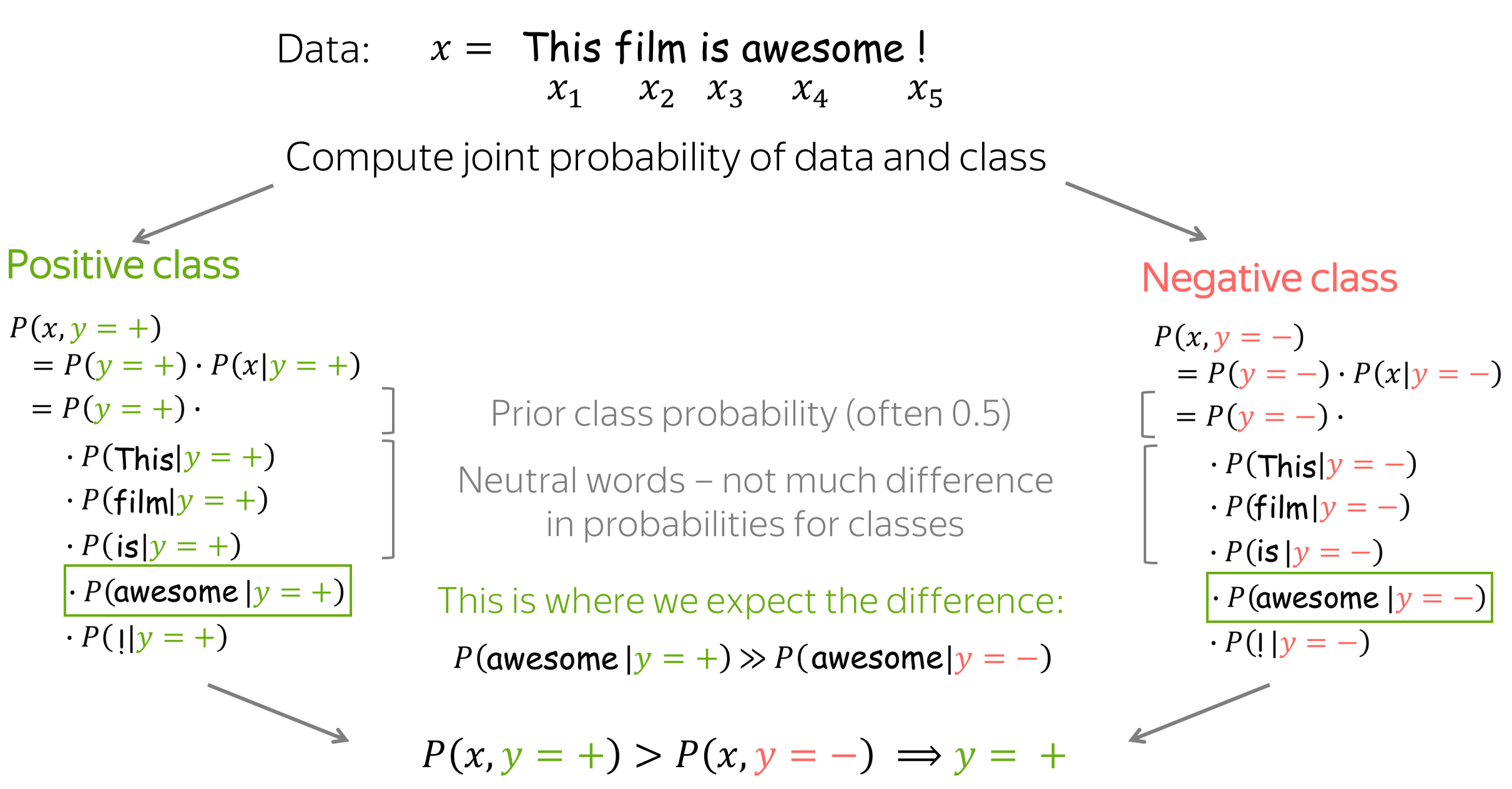
A high-level idea of the Naive Bayes approach is given below: we rewrite the conditional class probability \(P(y=k|x)\) using Bayes's rule and get \(P(x|y=k)\cdot P(y=k)\).
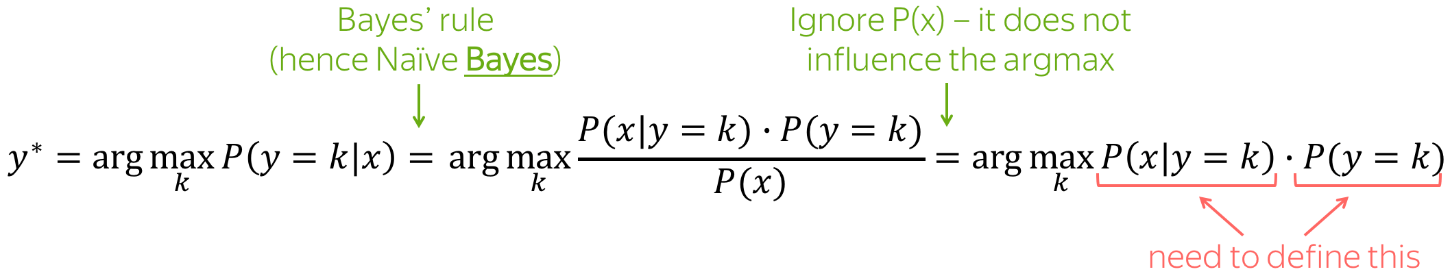
This is a generative model!
Naive Bayes is a generative model: it models the joint probability of data.
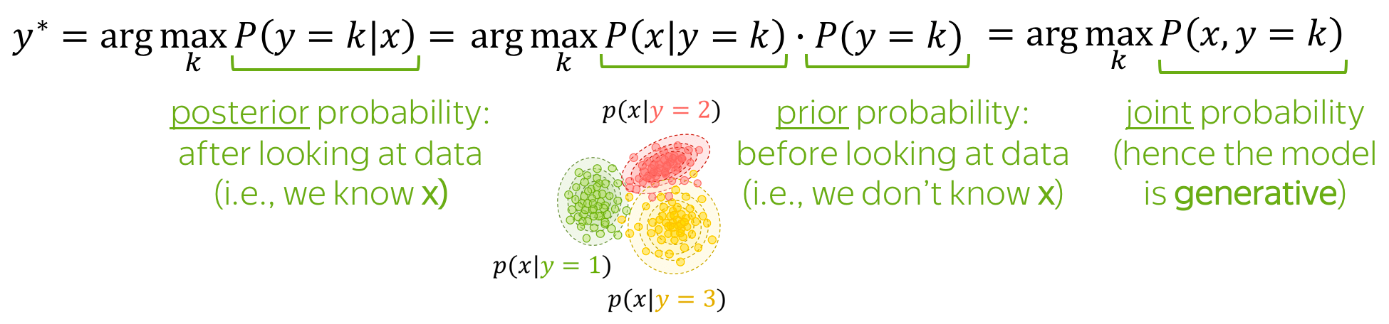
Note also the terminology:
- prior probability \(P(y=k)\): class probability before looking at data (i.e., before knowing \(x\));
- posterior probability \(P(y=k|x)\): class probability after looking at data (i.e., after knowing the specific \(x\));
- joint probability \(P(x, y)\): the joint probability of data (i.e., both examples \(x\) and labels \(y\));
- maximum a posteriori (MAP) estimate: we pick the class with the highest posterior probability.
How to define P(x|y=k) and P(y=k)?
P(y=k): count labels
\(P(y=k)\) is very easy to get: we can just evaluate the proportion of documents with the label \(k\) (this is the maximum likelihood estimate, MLE). Namely, \[P(y=k)=\frac{N(y=k)}{\sum\limits_{i}N(y=i)},\] where \(N(y=k)\) is the number of examples (documents) with the label \(k\).
P(x|y=k): use the "naive" assumptions, then count
Here we assume that document \(x\) is represented as a set of features, e.g., a set of its words \((x_1, \dots, x_n)\): \[P(x| y=k)=P(x_1, \dots, x_n|y=k).\]
The Naive Bayes assumptions are
- Bag of Words assumption: word order does not matter,
- Conditional Independence assumption: features (words) are independent given the class.
Intuitively, we assume that the probability of each word to appear in a document with class \(k\) does not depend on context (neither word order nor other words at all). For example, we can say that awesome, brilliant, great are more likely to appear in documents with a positive sentiment and awful, boring, bad are more likely in negative documents, but we know nothing about how these (or other) words influence each other.
With these "naive" assumptions we get: \[P(x| y=k)=P(x_1, \dots, x_n|y=k)=\prod\limits_{t=1}^nP(x_t|y=k).\] The probabilities \(P(x_i|y=k)\) are estimated as the proportion of times the word \(x_i\) appeared in documents of class \(k\) among all tokens in these documents: \[P(x_i|y=k)=\frac{N(x_i, y=k)}{\sum\limits_{t=1}^{|V|}N(x_t, y=k)},\] where \(N(x_i, y=k)\) is the number of times the token \(x_i\) appeared in documents with the label \(k\), \(V\) is the vocabulary (more generally, a set of all possible features).
What if \(N(x_i, y=k)=0\)? Need to avoid this!
What if \(N(x_i, y=k)=0\), i.e. in training we haven't seen the token \(x_i\) in the documents with class \(k\)? This will null out the probability of the whole document, and this is not what we want! For example, if we haven't seen some rare words (e.g., pterodactyl or abracadabra) in training positive examples, it does not mean that a positive document can never contain these words.
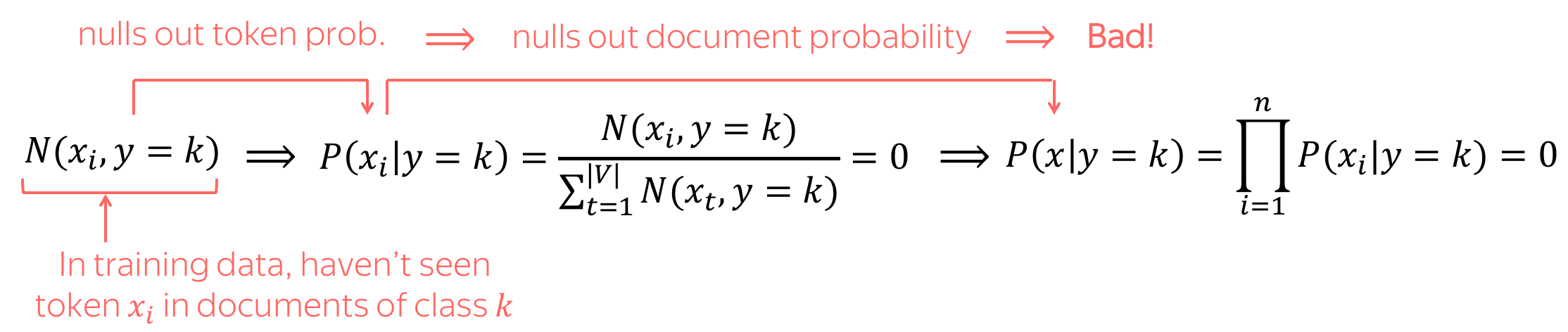
To avoid this, we'll use a simple trick: we add to counts of all words a small \(\delta\): \[P(x_i|y=k)=\frac{\color{red}{\delta} +\color{black} N(x_i, y=k) }{\sum\limits_{t=1}^{|V|}(\color{red}{\delta} +\color{black}N(x_t, y=k))} = \frac{\color{red}{\delta} +\color{black} N(x_i, y=k) }{\color{red}{\delta\cdot |V|}\color{black} + \sum\limits_{t=1}^{|V|}\color{black}N(x_t, y=k)} ,\] where \(\delta\) can be chosen using cross-validation.
Note: this is Laplace smoothing (aka Add-1 smoothing if \(\delta=1\)). We'll learn more about smoothings in the next lecture when talking about Language Modeling.
Making a Prediction
As we already mentioned, Naive Bayes (and, more broadly, generative models) make a prediction based on the joint probability of data and class: \[y^{\ast} = \arg \max\limits_{k}P(x, y=k) = \arg \max\limits_{k} P(y=k)\cdot P(x|y=k).\]
Intuitively, Naive Bayes expects that some words serve as class indicators. For example, for sentiment classification tokens awesome, brilliant, great will have higher probability given positive class then negative. Similarly, tokens awful, boring, bad will have higher probability given negative class then positive.
Final Notes on Naive Bayes
Practical Note: Sum of Log-Probabilities Instead of Product of Probabilities
The main expression Naive Bayes uses for classification is a product lot of probabilities: \[P(x, y=k)=P(y=k)\cdot P(x_1, \dots, x_n|y)=P(y=k)\cdot \prod\limits_{t=1}^nP(x_t|y=k).\] A product of many probabilities may be very unstable numerically. Therefore, usually instead of \(P(x, y)\) we consider \(\log P(x, y)\): \[\log P(x, y=k)=\log P(y=k) + \sum\limits_{t=1}^n\log P(x_t|y=k).\] Since we care only about argmax, we can consider \(\log P(x, y)\) instead of \(P(x, y)\).
Important! Note that in practice, we will usually deal with log-probabilities and not probabilities.
View in the General Framework
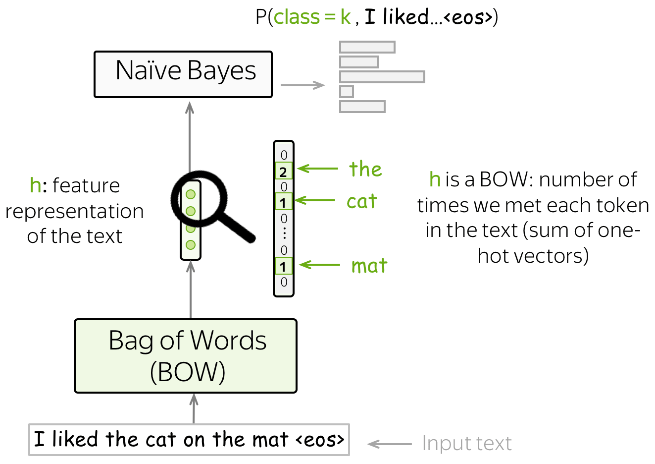
Remember our general view on the classification task? We obtain feature representation of the input text using some method, then use this feature representation for classification.
In Naive Bayes, our features are words, and the feature representation is the Bag-of-Words (BOW) representation - a sum of one-hot representations of words. Indeed, to evaluate \(P(x, y)\) we only need to count the number of times each token appeared in the text.
Feature Design
In the standard setting, we used words as features. However, you can use other types of features: URL, user id, etc.
Even if your data is a plain text (without fancy things such as URL, user id, etc), you can still design features in different ways. Learn how to improve Naive Bayes in this exercise in the Research Thinking section.
Maximum Entropy Classifier (aka Logistic Regression)
Differently from Naive Bayes, MaxEnt classifier is a discriminative model, i.e., we are interested in \(P(y=k|x)\) and not in the joint distribution \(p(x, y)\). Also, we will learn how to use features: this is in contrast to Naive Bayes, where we defined how to use the features ourselves.
Here we also have to define features manually, but we have more freedom: features do not have to be categorical (in Naive Bayes, they had to!). We can use the BOW representation or come up with something more interesting.
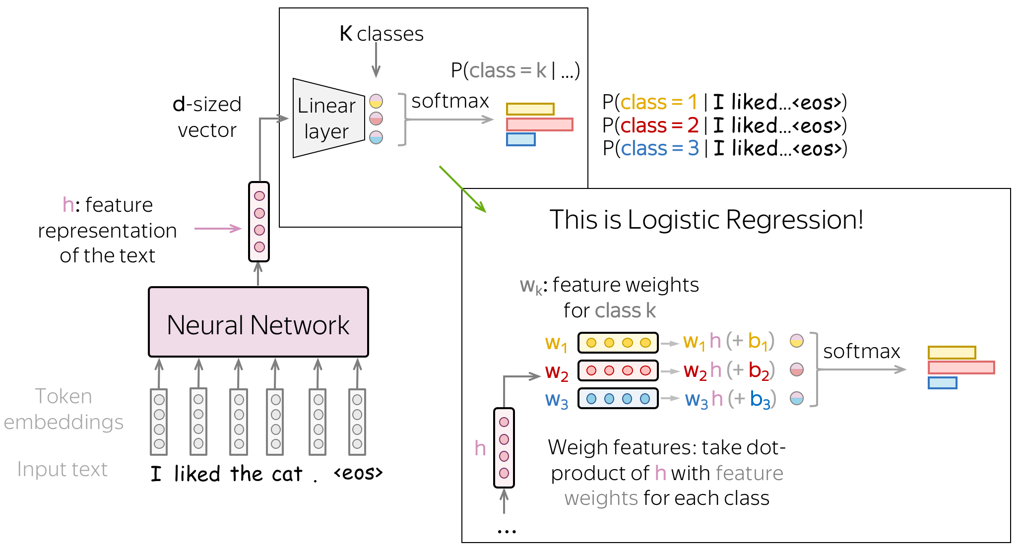
The general classification pipeline here is as follows:
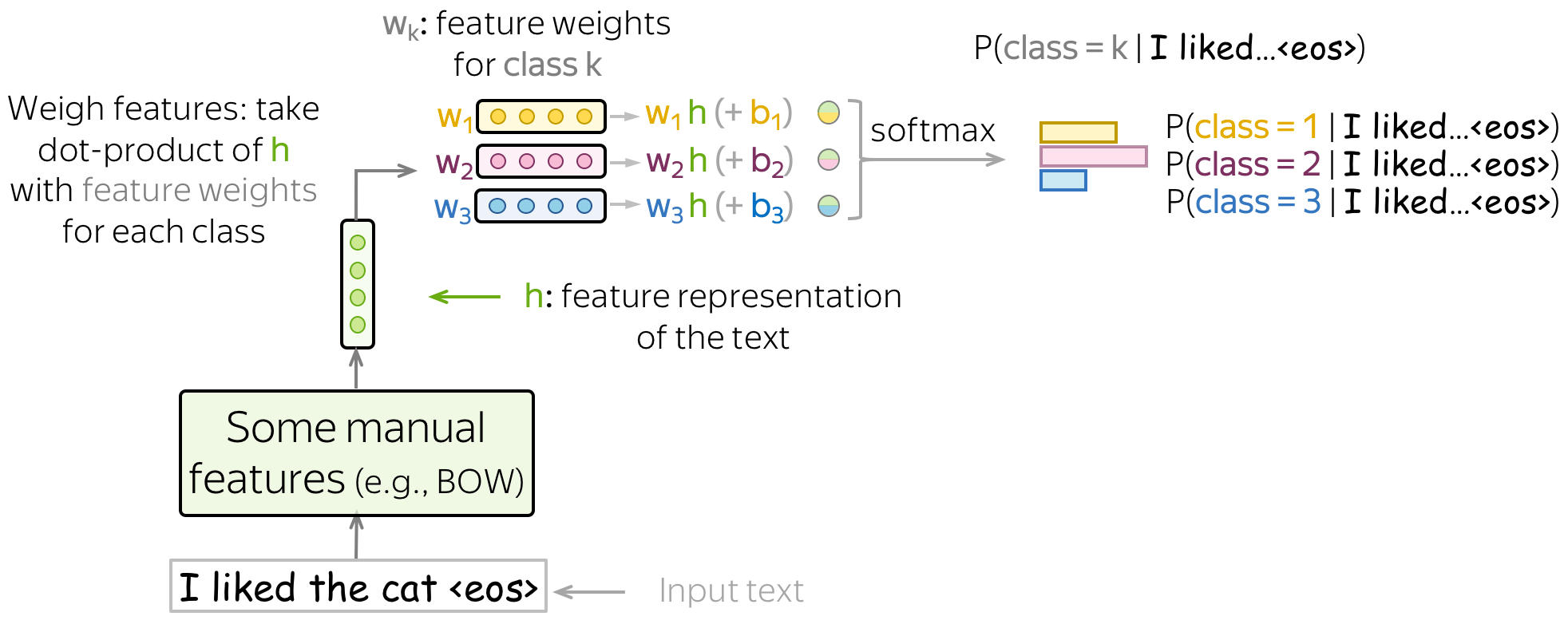
- get \(\color{#7aab00}{h}\color{black}=(\color{#7aab00}{f_1}\color{black}, \color{#7aab00}{f_2}\color{black}, \dots, \color{#7aab00}{f_n}\color{black}{)}\) - feature representation of the input text;
- take \(w^{(i)}=(w_1^{(i)}, \dots, w_n^{(i)})\) - vectors with feature weights for each of the classes;
- for each class, weigh features, i.e. take the dot product of feature representation \(\color{#7aab00}{h}\) with feature weights \(w^{(k)}\): \[w^{(k)}\color{#7aab00}{h}\color{black} = w_1^{(k)}\cdot\color{#7aab00}{f_1}\color{black}+\dots+ w_n^{(k)}\cdot\color{#7aab00}{f_n}\color{black}{, \ \ \ \ \ k=1, \dots, K.} \] To get a bias term in the sum above, we define one of the features being 1 (e.g., \(\color{#7aab00}{f_0}=1\)). Then \[w^{(k)}\color{#7aab00}{h}\color{black} = \color{red}{w_0^{(k)}}\color{black} + w_1^{(k)}\cdot\color{#7aab00}{f_1}\color{black}+\dots+ w_n^{(k)}\cdot\color{#7aab00}{f_{n}}\color{black}{, \ \ \ \ \ k=1, \dots, K.} \]
- get class probabilities using softmax: \[P(class=k|\color{#7aab00}{h}\color{black})= \frac{\exp(w^{(k)}\color{#7aab00}{h}\color{black})}{\sum\limits_{i=1}^K \exp(w^{(i)}\color{#7aab00}{h}\color{black})}.\] Softmax normalizes the \(K\) values we got at the previous step to a probability distribution over output classes.
Look at the illustration below (classes are shown in different colors).
Training: Maximum Likelihood Estimate
Given training examples \(x^1, \dots, x^N\) with labels \(y^1, \dots, y^N\), \(y^i\in\{1, \dots, K\}\), we pick those weights \(w^{(k)}, k=1..K\) which maximize the probability of the training data: \[w^{\ast}=\arg \max\limits_{w}\sum\limits_{i=1}^N\log P(y=y^i|x^i).\] In other words, we choose parameters such that the data is more likely to appear. Therefore, this is called the Maximum Likelihood Estimate (MLE) of the parameters.
To find the parameters maximizing the data log-likelihood, we use gradient ascent: gradually improve weights during multiple iterations over the data. At each step, we maximize the probability a model assigns to the correct class.
Equvalence to minimizing cross-entropy
Note that maximizing data log-likelihood is equivalent to minimizing cross entropy between the target probability distribution \(p^{\ast} = (0, \dots, 0, 1, 0, \dots)\) (1 for the target label, 0 for the rest) and the predicted by the model distribution \(p=(p_1, \dots, p_K), p_i=p(i|x)\): \[Loss(p^{\ast}, p^{})= - p^{\ast} \log(p) = -\sum\limits_{i=1}^{K}p_i^{\ast} \log(p_i).\] Since only one of \(p_i^{\ast}\) is non-zero (1 for the target label \(k\), 0 for the rest), we will get \(Loss(p^{\ast}, p) = -\log(p_{k})=-\log(p(k| x)).\)
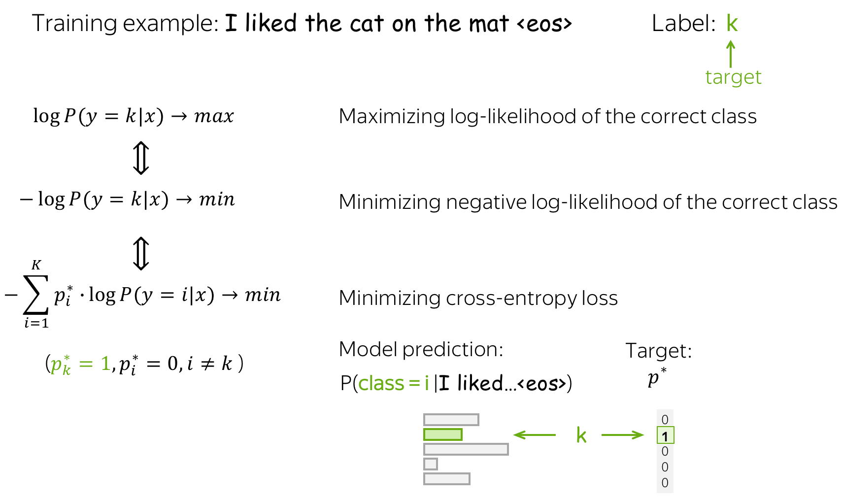
This equivalence is very important for you to understand: when talking about neural approaches, people usually say that they minimize the cross-entropy loss. Do not forget that this is the same as maximizing the data log-likelihood.
Naive Bayes vs Logistic Regression
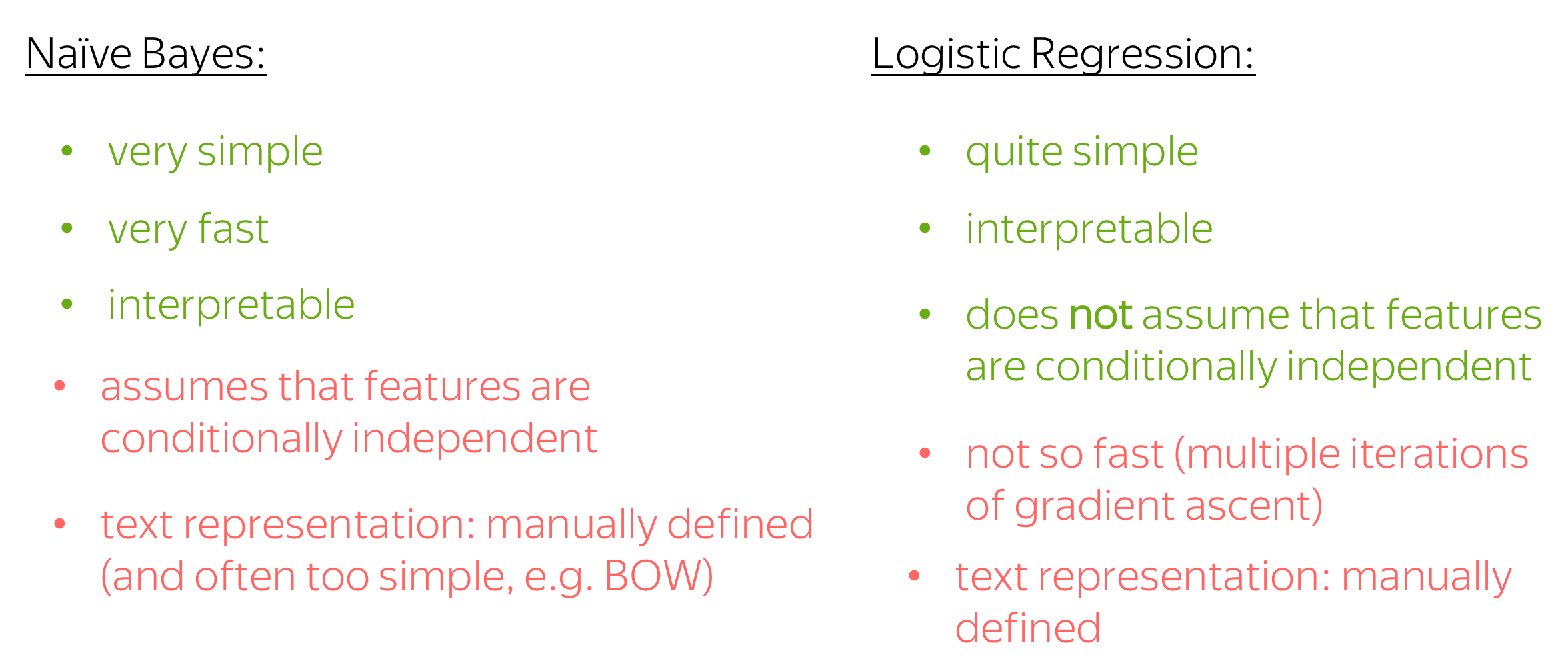
Let's finalize this part by discussing the advantages and drawbacks of logistic regression and Naive Bayes.
- simplicity
Both methods are simple; Naive Bayes is the simplest one. - interpretability
Both methods are interpretable: you can look at the features which influenced the predictions most (in Naive Bayes - usually words, in logistic regression - whatever you defined). - training speed
Naive Bayes is very fast to train - it requires only one pass through the training data to evaluate the counts. For logistic regression, this is not the case: you have to go over the data many times until the gradient ascent converges. - independence assumptions
Naive Bayes is too "naive" - it assumed that features (words) are conditionally independent given class. Logistic regression does not make this assumption - we can hope it is better. - text representation: manual
Both methods use manually defined feature representation (in Naive Bayes, BOW is the standard choice, but you still choose this yourself). While manually defined features are good for interpretability, they may be no so good for performance - you are likely to miss something which can be useful for the task.
SVM for Text Classification
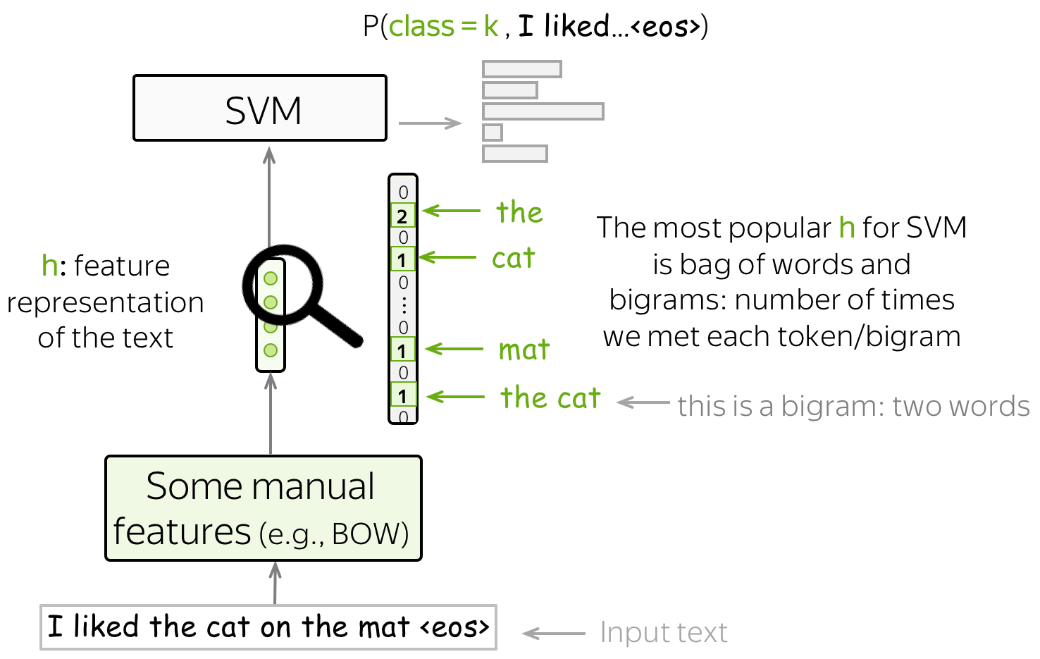
One more method for text classification based on manually designed features is SVM. The most basic (and popular) features for SVMs are bag-of-words and bag-of-ngrams (ngram is a tuple of n words). With these simple features, SVMs with linear kernel perform better than Naive Bayes (see, for example, the paper Question Classification using Support Vector Machines).
Text Classification with Neural Networks
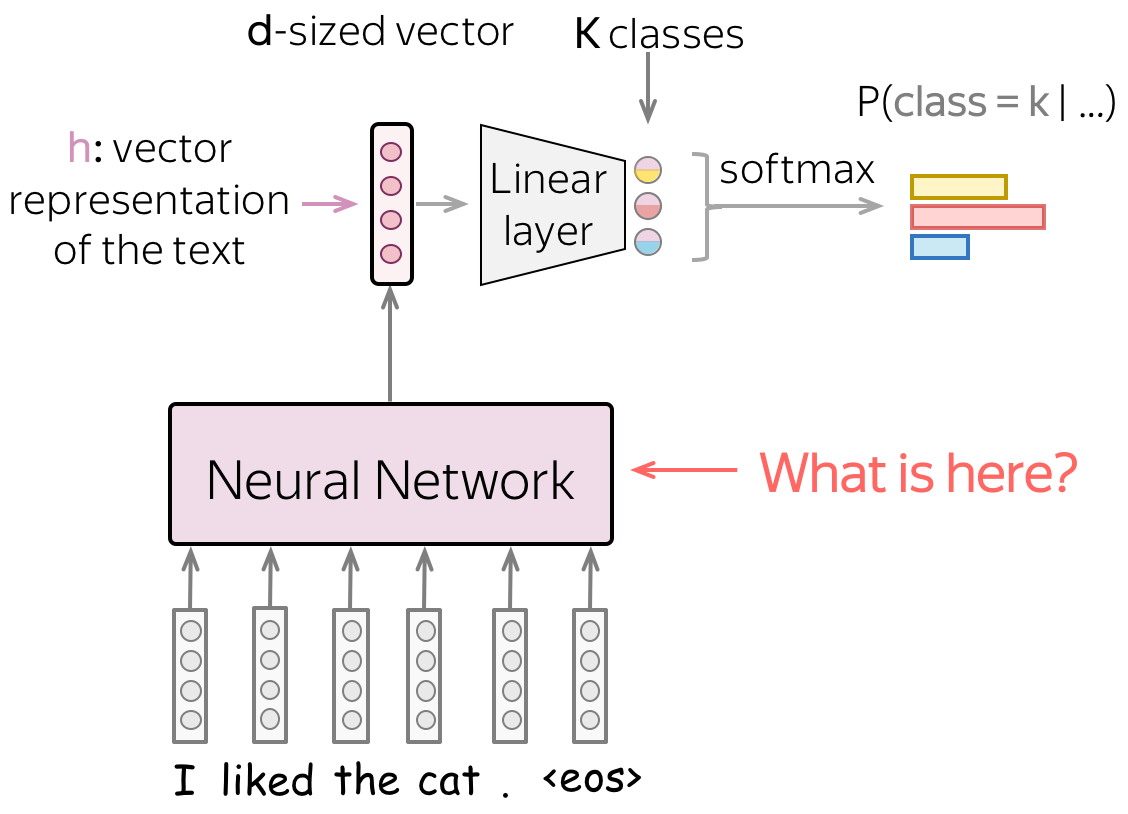
Instead of manually defined features, let a neural network to learn useful features.
The main idea of neural-network-based classification is that feature representation of the input text can be obtained using a neural network. In this setting, we feed the embeddings of the input tokens to a neural network, and this neural network gives us a vector representation of the input text. After that, this vector is used for classification.
When dealing with neural networks, we can think about the classification part (i.e., how to get class probabilities from a vector representation of a text) in a very simple way.
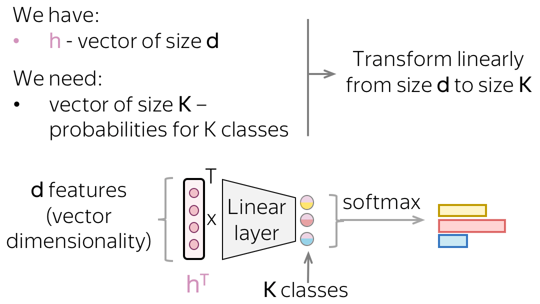
Vector representation of a text has some dimensionality \(d\), but in the end, we need a vector of size \(K\) (probabilities for \(K\) classes). To get a \(K\)-sized vector from a \(d\)-sized, we can use a linear layer. Once we have a \(K\)-sized vector, all is left is to apply the softmax operation to convert the raw numbers into class probabilities.
Classification Part: This is Logistic Regression!
Let us look closer to the neural network classifier. The way we use vector representation of the input text is exactly the same as we did with logistic regression: we weigh features according to feature weights for each class. The only difference from logistic regression is where the features come from: they are either defined manually (as we did before) or obtained by a neural network.
Intuition: Text Representation Points in the Direction of Class Representation
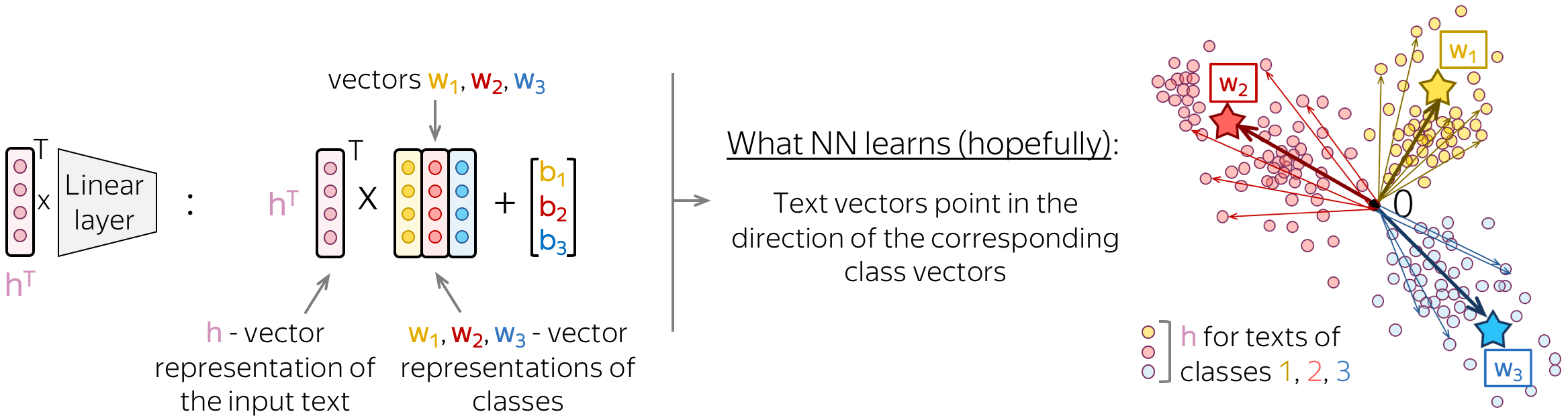
If we look at this final linear layer more closely, we will see that the columns of its matrix are vectors \(w_i\). These vectors can be thought of as vector representations of classes. A good neural network will learn to represent input texts in such a way that text vectors will point in the direction of the corresponding class vectors.
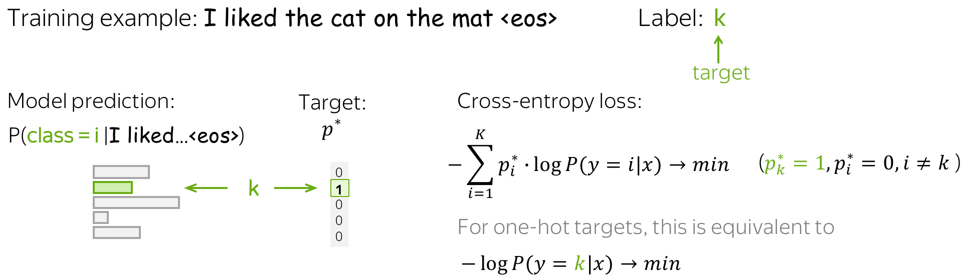
Training and the Cross-Entropy Loss
Neural classifiers are trained to predict probability distributions over classes. Intuitively, at each step we maximize the probability a model assigns to the correct class.
The standard loss function is the cross-entropy loss. Cross-entropy loss for the target probability distribution \(p^{\ast} = (0, \dots, 0, 1, 0, \dots)\) (1 for the target label, 0 for the rest) and the predicted by the model distribution \(p=(p_1, \dots, p_K), p_i=p(i|x)\): \[Loss(p^{\ast}, p^{})= - p^{\ast} \log(p) = -\sum\limits_{i=1}^{K}p_i^{\ast} \log(p_i).\] Since only one of \(p_i^{\ast}\) is non-zero (1 for the target label \(k\), 0 for the rest), we will get \(Loss(p^{\ast}, p) = -\log(p_{k})=-\log(p(k| x)).\) Look at the illustration for one training example.
In training, we gradually improve model weights during multiple iterations over the data: we iterate over training examples (or batches of examples) and make gradient updates. At each step, we maximize the probability a model assigns to the correct class. At the same time, we minimize sum of the probabilities of incorrect classes: since sum of all probabilities is constant, by increasing one probability we decrease sum of all the rest (Lena: Here I usually imagine a bunch of kittens eating from the same bowl: one kitten always eats at the expense of the others).
Look at the illustration of the training process.
Recap: This is equivalent to maximizing the data likelihood
Do not forget that when talking about MaxEnt classifier (logistic regression), we showed that minimizing cross-entropy is equivalent to maximizing the data likelihood. Therefore, here we are also trying to get the Maximum Likelihood Estimate (MLE) of model parameters.
Models for Text Classification
We need a model that can produce a fixed-sized vector for inputs of different lengths.
In this part, we will look at different ways to get a vector representation of an input text using neural networks. Note that while input texts can have different lengths, the vector representation of a text has to have a fixed size: otherwise, a network will not "work".
We begin with the simplest approaches which use only word embeddings (without adding a model on top of that). Then we look at recurrent and convolutional networks.
Lena: A bit later in the course, you will learn about Transformers and the most recent classification techniques using large pretrained models.
Basics: Bag of Embeddings (BOE) and Weighted BOE
The simplest you can do is use only word embeddings without any neural network on top of that. To get vector representation of a text, we can either sum all token embeddings (Bag of Embeddings) or use a weighted sum of these embeddings (with weights, for example, being tf-idf or something else).
Bag of Embeddings (ideally, along with Naive Bayes) should be a baseline for any model with a neural network: if you can't do better than that, it's not worth using NNs at all. This can be the case if you don't have much data.
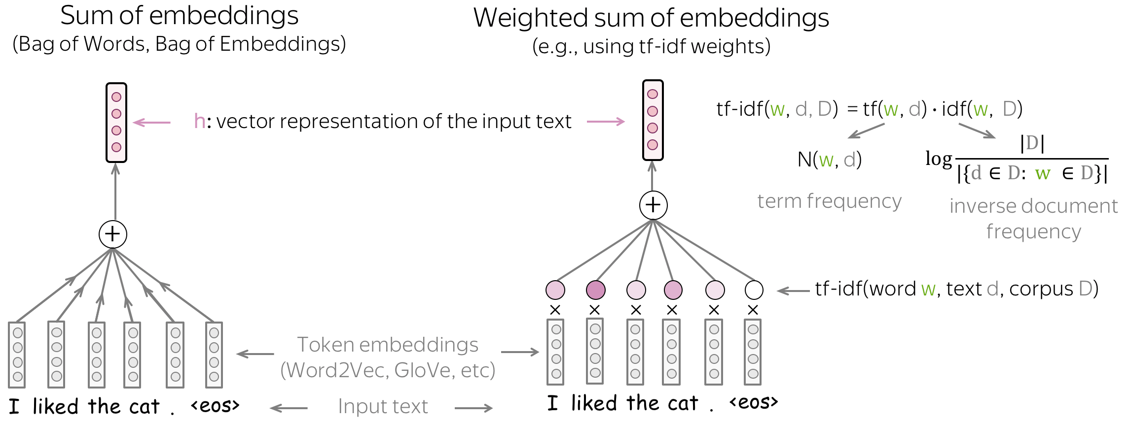
While Bag of Embeddings (BOE) is sometimes called Bag of Words (BOW), note that these two are very different. BOE is the sum of embeddings and BOW is the sum of one-hot vectors: BOE knows a lot more about language. The pretrained embeddings (e.g., Word2Vec or GloVe) understand similarity between words. For example, awesome, brilliant, great will be represented with unrelated features in BOW but similar word vectors in BOE.
Note also that to use a weighted sum of embeddings, you need to come up with a way to get weights. However, this is exactly what we wanted to avoid by using neural networks: we don't want to introduce manual features, but rather let a network to learn useful patterns.
Bag of Embeddings as Features for SVM
You can use SVM on top of BOE! The only difference from SVMs in classical approaches (on top of bag-of-words and bag-of-ngrams) if the choice of a kernel: here the RBF kernel is better.
Models: Recurrent (RNN/LSTM/etc)
Recurrent networks are a natural way to process text in a sense that, similar to humans, they "read" a sequence of tokens one by one and process the information. Hopefully, at each step the network will "remember" everything it has read before.
Basics: Recurrent Neural Networks
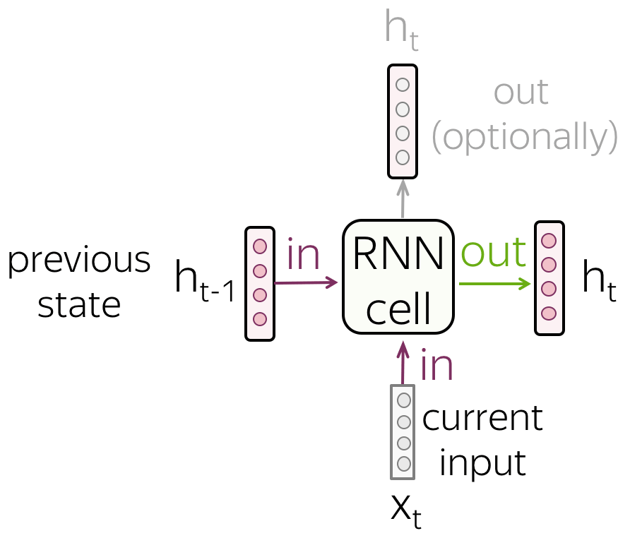
• RNN cell
At each step, a recurrent network receives a new input vector (e.g., token embedding) and the previous network state (which, hopefully, encodes all previous information). Using this input, the RNN cell computes the new state which it gives as output. This new state now contains information about both current input and the information from previous steps.
• RNN reads a sequence of tokens
Look at the illustration: RNN reads a text token by token, at each step using a new token embedding and the previous state.
Note that the RNN cell is the same at each step!
• Vanilla RNN
The simplest recurrent network, Vanilla RNN, transforms \(h_{t-1}\) and \(x_t\) linearly, then applies a non-linearity (most often, the \(\tanh\) function): \[h_t = \tanh(h_{t-1}W_h + x_tW_t).\]
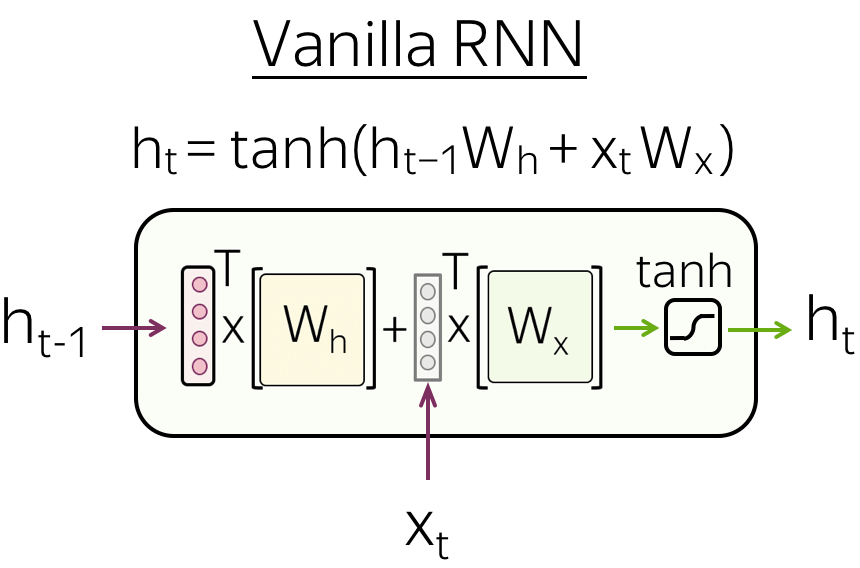
Vanilla RNNs suffer from the vanishing and exploding gradients problem. To alleviate this problem, more complex recurrent cells (e.g., LSTM, GRU, etc) perform several operations on the input and use gates. For more details of RNN basics, look at the Colah's blog post.
Recurrent Neural Networks for Text Classification
Here we (finally!) look at how we can use recurrent models for text classification. Everything you will see here will apply to all recurrent cells, and by "RNN" in this part I refer to recurrent cells in general (e.g. vanilla RNN, LSTM, GRU, etc).
Let us recall what we need:
We need a model that can produce a fixed-sized vector for inputs of different lengths.
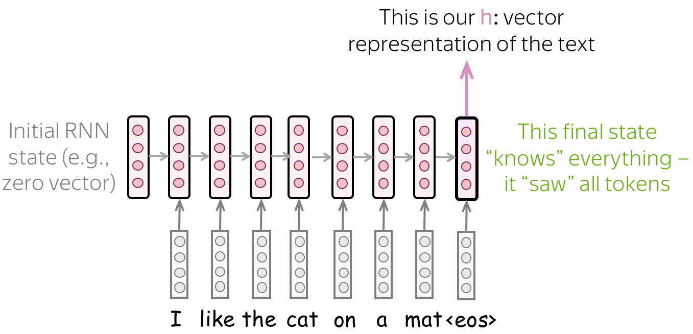
• Simple: read a text, take the final state
The most simple recurrent model is a one-layer RNN network. In this network, we have to take the state which knows more about input text. Therefore, we have to use the last state - only this state saw all input tokens.
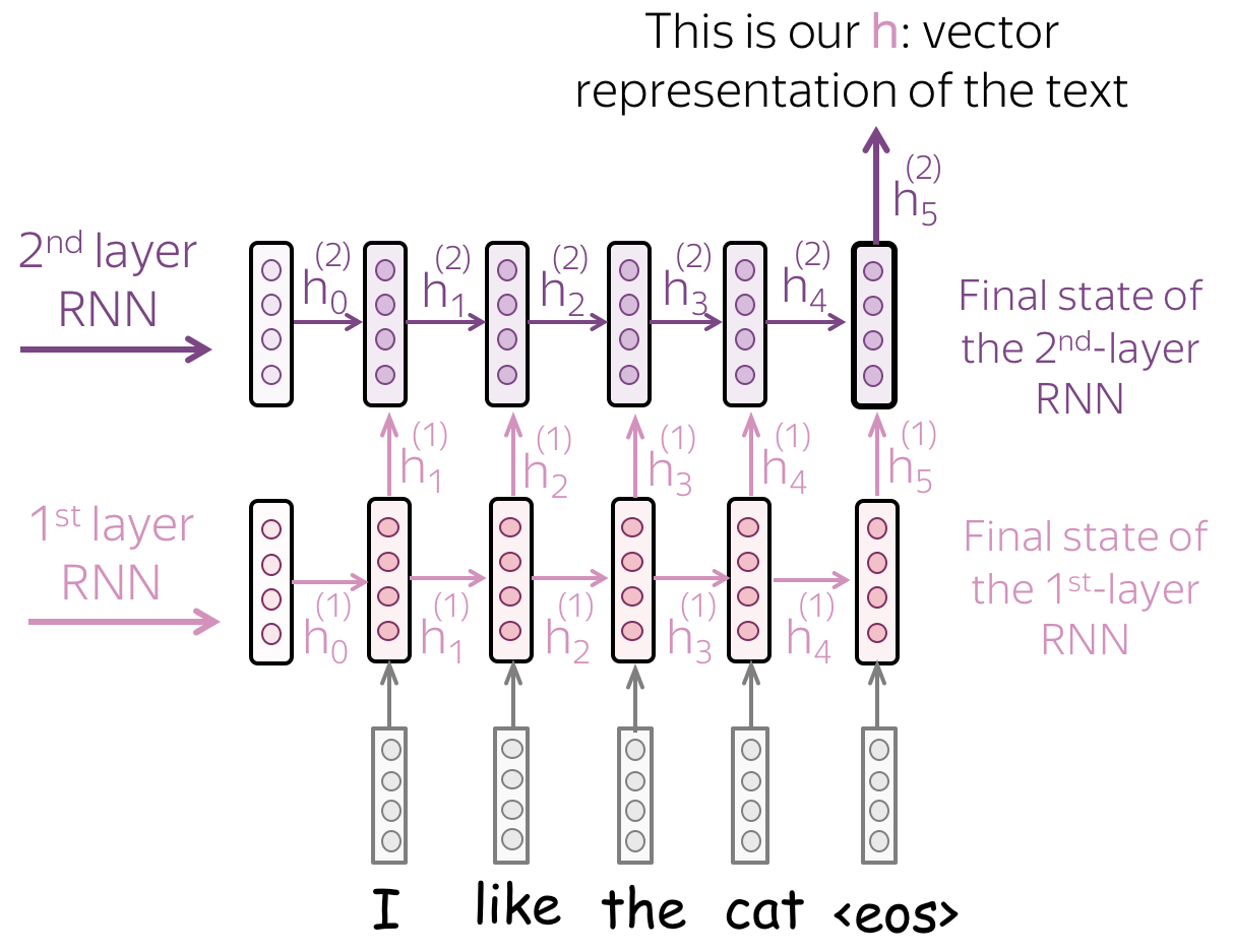
• Multiple layers: feed the states from one RNN to the next one
To get a better text representation, you can stack multiple layers. In this case, inputs for the higher RNN are representations coming from the previous layer.
The main hypothesis is that with several layers, lower layers will catch local phenomena (e.g., phrases), while higher layers will be able to learn more high-level things (e.g., topic).
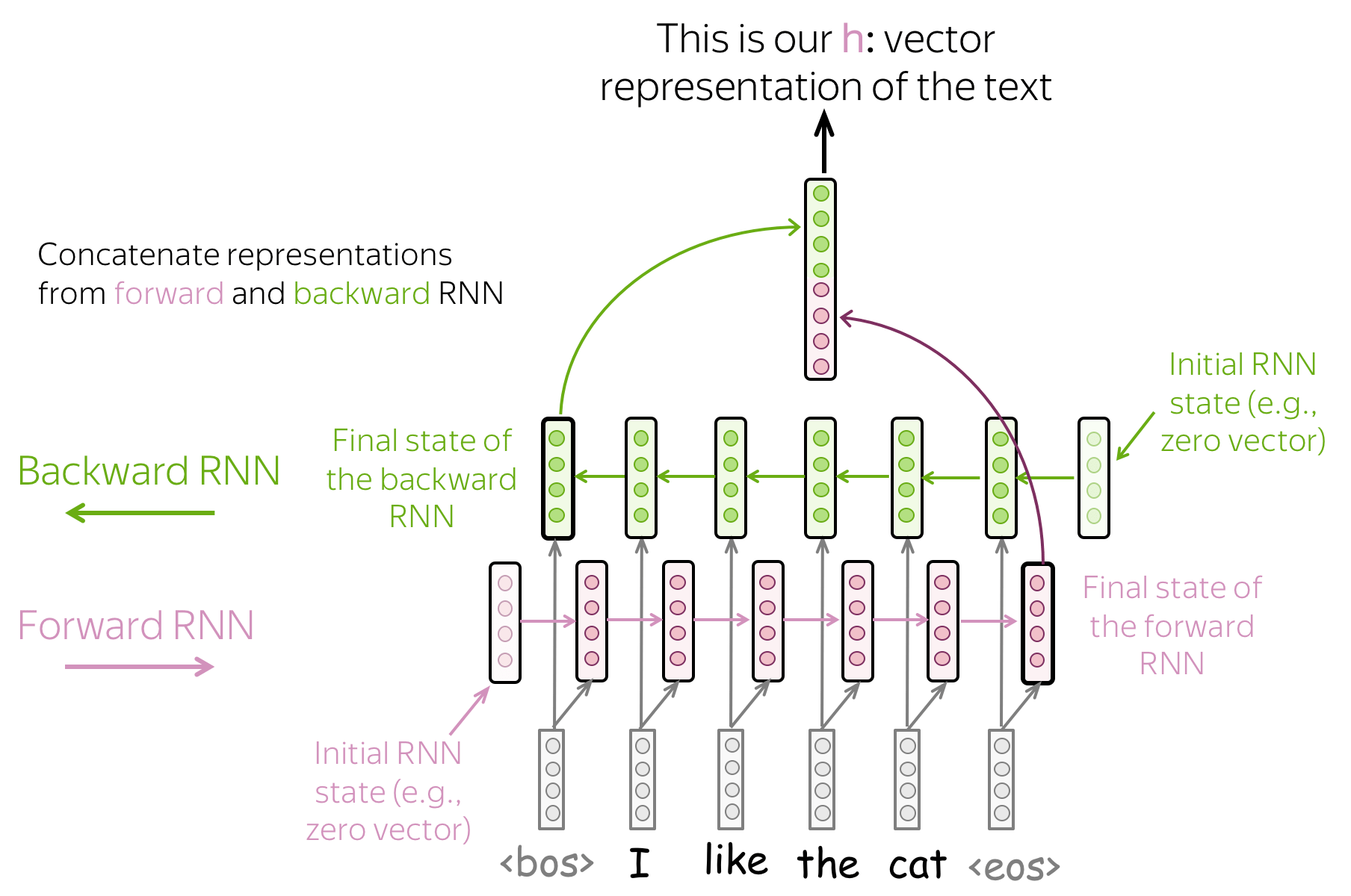
• Bidirectional: use final states from forward and backward RNNs.
Previous approaches may have a problem: the last state can easily "forget" earlier tokens. Even strong models such as LSTMs can still suffer from that!
To avoid this, we can use two RNNs: forward, which reads input from left to right, and backward, which reads input from right to left. Then we can use the final states from both models: one will better remember the final part of a text, another - the beginning. These states can be concatenated, or summed, or something else - it's your choice!
• Combinations: do everything you want!
You can combine the ideas above. For example, in a multi-layered network, some layers can go in the opposite direction, etc.
Models: Convolutional (CNN)
The detailed description of convolutional models in general is in Convolutional Models Supplementary. In this part, we consider only convolutions for text classification.
Convolutions for Images and Translation Invariance
Convolutional networks were originally developed for computer vision tasks. Therefore, let's first understand the intuition behind convolutional models for images.
Imagine we want to classify an image into several classes, e.g. cat, dog, airplane, etc. In this case, if you find a cat on an image, you don't care where on the image this cat is: you care only that it is there somewhere.
Convolutional networks apply the same operation to small parts of an image: this is how they extract features. Each operation is looking for a match with a pattern, and a network learns which patterns are useful. With a lot of layers, the learned patterns become more and more complicated: from lines in the early layers to very complicated patterns (e.g., the whole cat or dog) on the upper ones. You can look at the examples in the Analysis and Interpretability section.
This property is called translation invariance: translation because we are talking about shifts in space, invariance because we want it to not matter.
The illustration is adapted from the one taken from
this cool repo.
Convolutions for Text
Well, for images it's all clear: e.g. we want to be able to move a cat because we don't care where the cat is. But what about texts? At first glance, this is not so straightforward: we can not move phrases easily - the meaning will change or we will get something that does not make much sense.
However, there are some applications where we can think of the same intuition. Let's imagine that we want to classify texts, but not cats/dogs as in images, but positive/negative sentiment. Then there are some words and phrases which could be very informative "clues" (e.g. it's been great, bored to death, absolutely amazing, the best ever, etc), and others which are not important at all. We don't care much where in a text we saw bored to death to understand the sentiment, right?
A Typical Model: Convolution+Pooling Blocks
Following the intuition above, we want to detect some patterns, but we don't care much where exactly these patterns are. This behavior is implemented with two layers:
- convolution: finds matches with patterns (as the cat head we saw above);
- pooling: aggregates these matches over positions (either locally or globally).
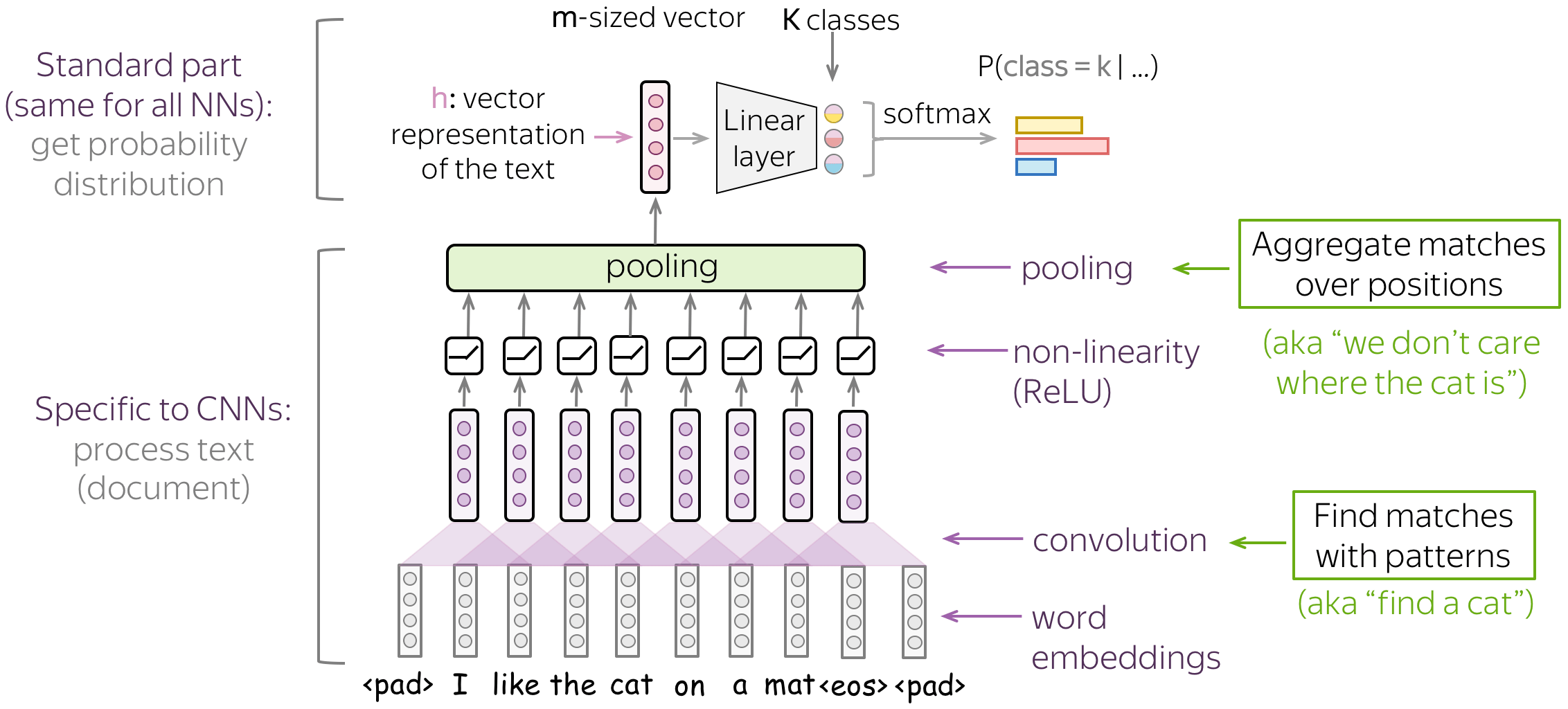
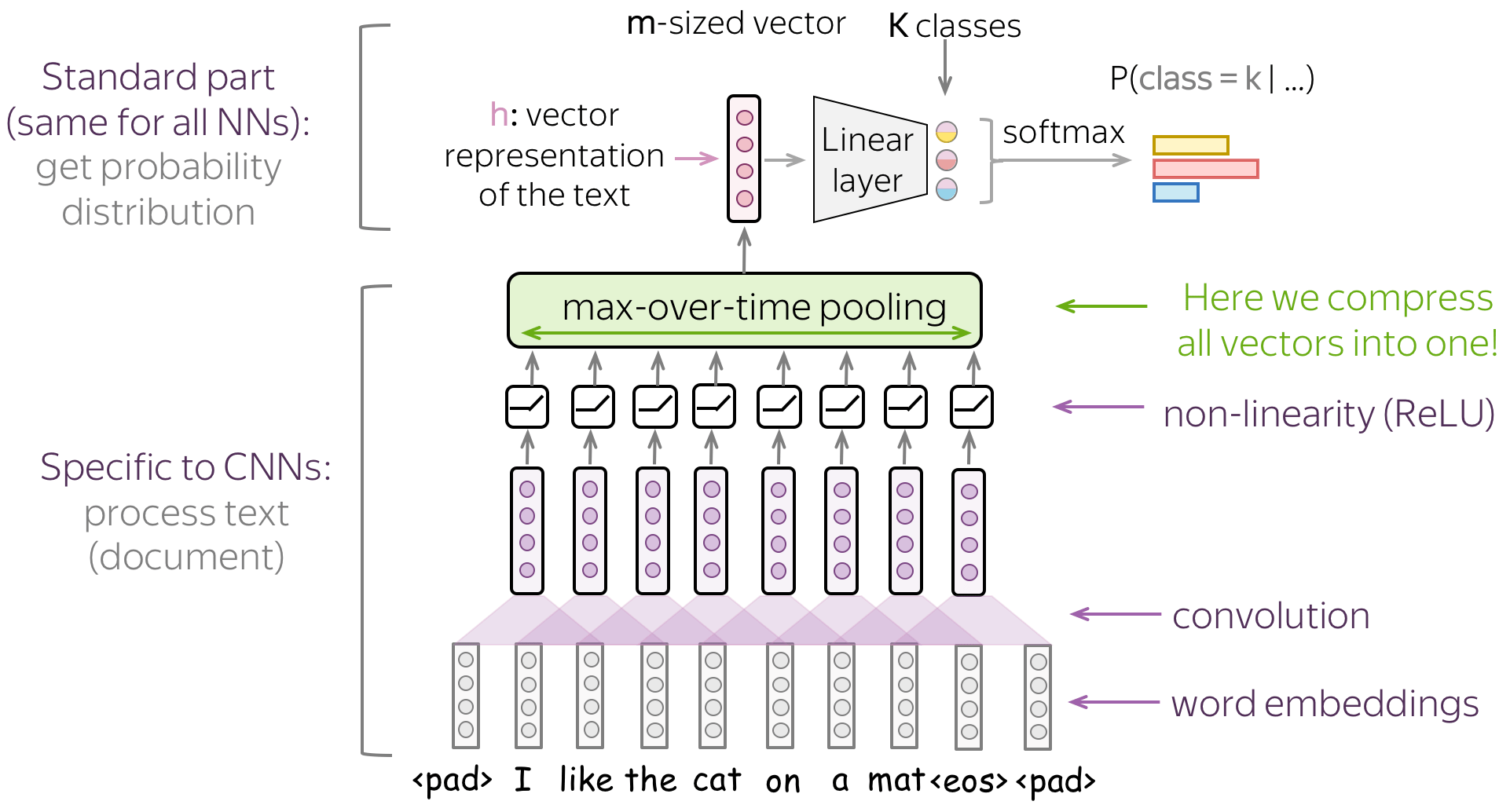
A typical convolutional model for text classification is shown on the figure. To get a vector representation of an input text, a convolutional layer is applied to word embedding, which is followed by a non-linearity (usually ReLU) and a pooling operation. The way this representation is used for classification is similar to other networks.
In the following, we discuss in detail the main building blocks, convolution and pooling, then consider modeling modifications.
Basics: Convolution Layer for Text
Convolutional Neural Networks were initially developed for computer vision tasks, e.g. classification of images (cats vs dogs, etc). The idea of a convolution is to go over an image with a sliding window and to apply the same operation, convolution filter, to each window.
The illustration (taken from this cool repo) shows this process for one filter: the bottom is the input image, the top is the filter output. Since an image has two dimensions (width and height), the convolution is two-dimensional.
Convolution filter for images. The illustration is from
this cool repo.
Differently from images, texts have only one dimension: here a convolution is one-dimensional: look at the illustration.
Convolution filter for text.
Convolution is a Linear Operation Applied to Each Window
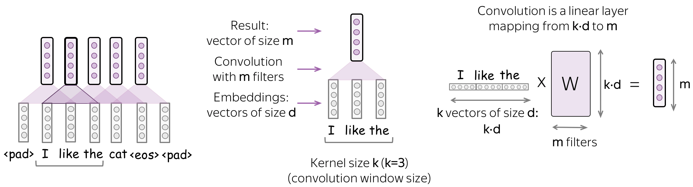
A convolution is a linear layer (followed by a non-linearity) applied to each input window. Formally, let us assume that
- \((x_1, \dots, x_n)\) - representations of the input words, \(x_i\in \mathbb{R}^d\);
- \(d\) (input channels) - size of an input embedding;
- \(k\) (kernel size) - the length of a convolution window (on the illustration, \(k=3\));
- \(m\) (output channels) - number of convolution filters (i.e., number of channels produced by the convolution).
Then a convolution is a linear layer \(W\in\mathbb{R}^{(k\cdot d)\times m}\). For a \(k\)-sized window \((x_i, \dots x_{i+k-1})\), the convolution takes the concatenation of these vectors \[u_i = [x_i, \dots x_{i+k-1}]\in\mathbb{R}^{k\cdot d}\] and multiplies by the convolution matrix: \[F_i = u_i \times W.\] A convolution goes over an input with a sliding window and applies the same linear transformation to each window.
Intuition: Each Filter Extracts a Feature
Intuitively, each filter in a convolution extracts a feature.
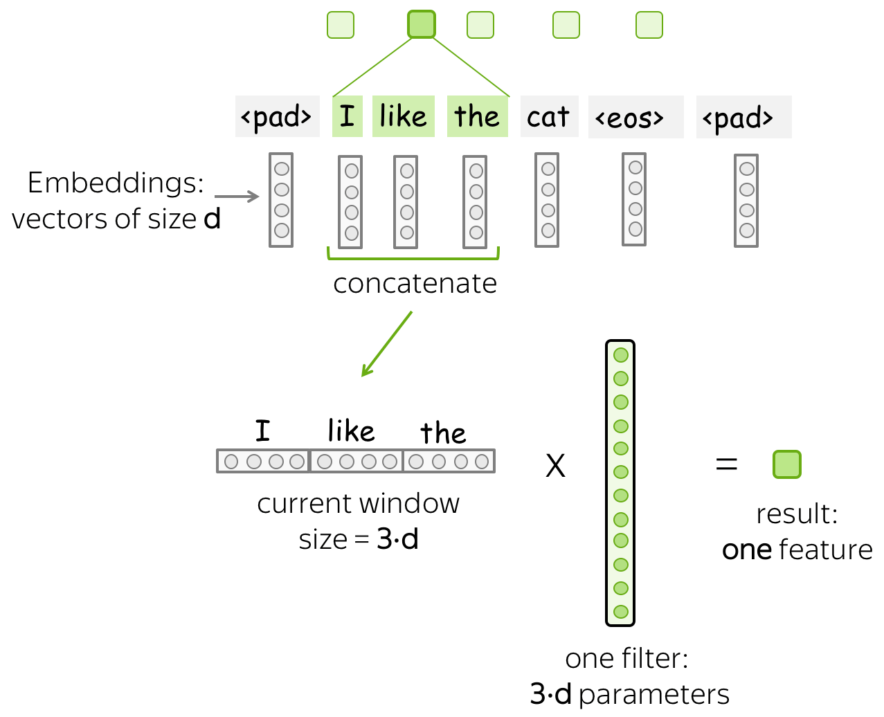
• One filter - one feature extractor
A filter takes vector representations in a current window and transforms them linearly into a single feature. Formally, for a window \(u_i = [x_i, \dots x_{i+k-1}]\in\mathbb{R}^{k\cdot d}\) a filter \(f\in\mathbb{R}^{k\cdot d}\) computes dot product: \[F_i^{(f)} = (f, u_i).\] The number \(F_i^{(f)}\) (the extracted "feature") is a result of applying the filter \(f\) to the window \((x_i, \dots x_{i+k-1})\).
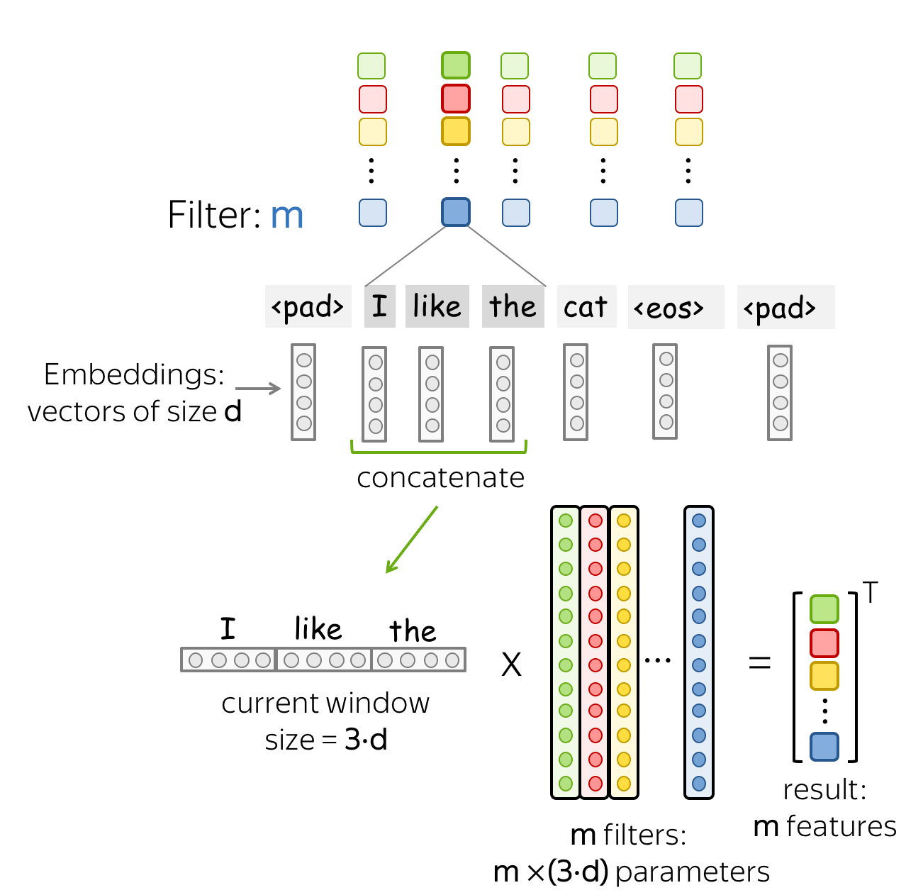
• m filters: m feature extractors
One filter extracts a single feature. Usually, we want many features: for this, we have to take several filters. Each filter reads an input text and extracts a different feature - look at the illustration. The number of filters is the number of output features you want to get. With \(m\) filters instead of one, the size of the convolutional layer we discussed above will become \((k\cdot d)\times m\).
This is done in parallel! Note that while I show you how a CNN "reads" a text, in practice these computations are done in parallel.
Basics: Pooling Operation
After a convolution extracted \(m\) features from each window, a pooling layer summarises the features in some region. Pooling layers are used to reduce the input dimension, and, therefore, to reduce the number of parameters used by the network.
• Max and Mean Pooling
The most popular is max-pooling: it takes maximum over each dimension, i.e. takes the maximum value of each feature.
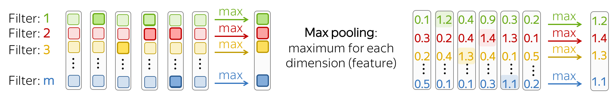
Intuitively, each feature "fires" when it sees some pattern: a visual pattern in an image (line, texture, a cat's paw, etc) or a text pattern (e.g., a phrase). After a pooling operation, we have a vector saying which of these patterns occurred in the input.
Mean-pooling works similarly but computes mean over each feature instead of maximum.
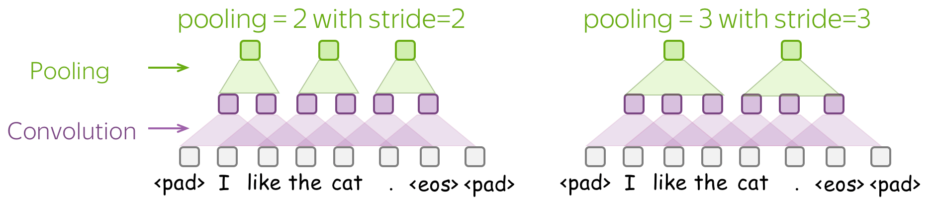
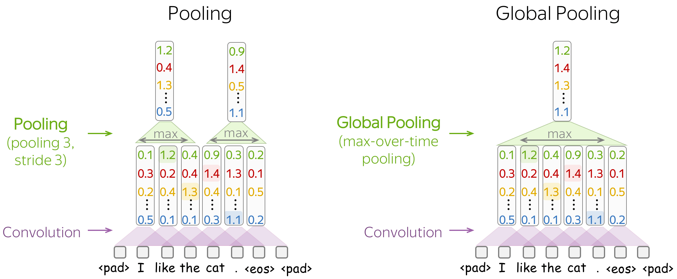
• Pooling and Global Pooling
Similarly to convolution, pooling is applied to windows of several elements. Pooling also has the stride parameter, and the most common approach is to use pooling with non-overlapping windows. For this, you have to set the stride parameter the same as the pool size. Look at the illustration.
The difference between pooling and global pooling is that pooling is applied over features in each window independently, while global pooling performs over the whole input. For texts, global pooling is often used to get a single vector representing the whole text; such global pooling is called max-over-time pooling, where the "time" axis goes from the first input token to the last.
Convolutional Neural Networks for Text Classification
Now, when we understand how the convolution and pooling work, let's come to modeling modifications. First, let us recall what we need:
We need a model that can produce a fixed-sized vector for inputs of different lengths.
Therefore, we need to construct a convolutional model that represents a text as a single vector.
The basic convolutional model for text classification is shown on the figure. It is almost the same as we saw before: the only thing that's changed is that we specified the type of pooling used. Specifically, after the convolution, we use global-over-time pooling. This is the key operation: it allows to compress a text into a single vector. The model itself can be different, but at some point it has to use the global pooling to compress input in a single vector.
• Several Convolutions with Different Kernel Sizes
Instead of picking one kernel size for your convolution, you can use several convolutions with different kernel sizes. The recipe is simple: apply each convolution to the data, add non-linearity and global pooling after each of them, then concatenate the results (on the illustration, non-linearity is omitted for simplicity). This is how you get vector representation of the data which is used for classification.
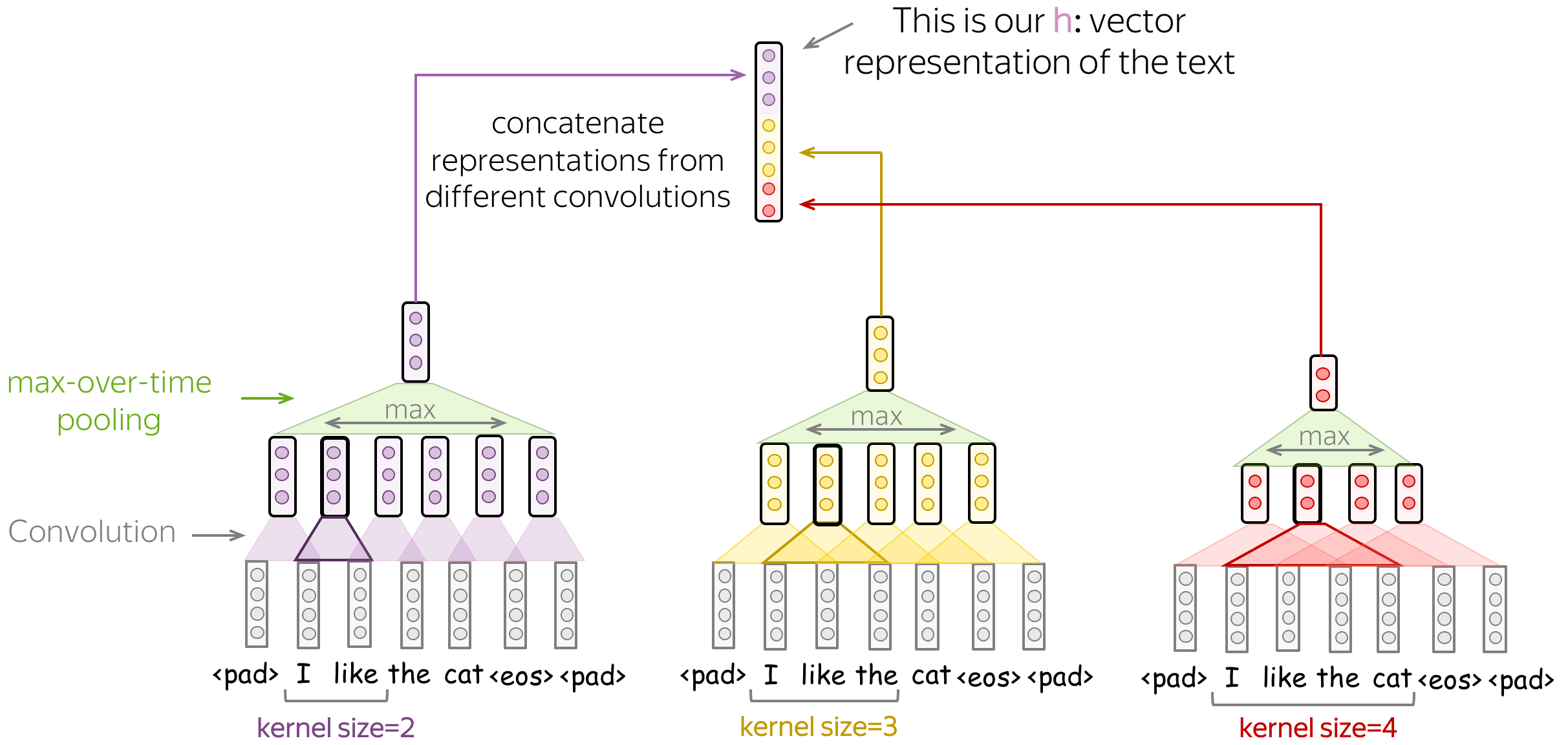
This idea was used, among others, in the paper Convolutional Neural Networks for Sentence Classification and many follow-ups.
• Stack Several Blocks Convolution+Pooling
Instead of one layer, you can stack several blocks convolution+pooling on top of each other. After several blocks, you can apply another convolution, but with global pooling this time. Remember: you have to get a single fixed-sized vector - for this, you need global pooling.
Such multi-layered convolutions can be useful when your texts are very long; for example, if your model is character-level (as opposed to word-level).
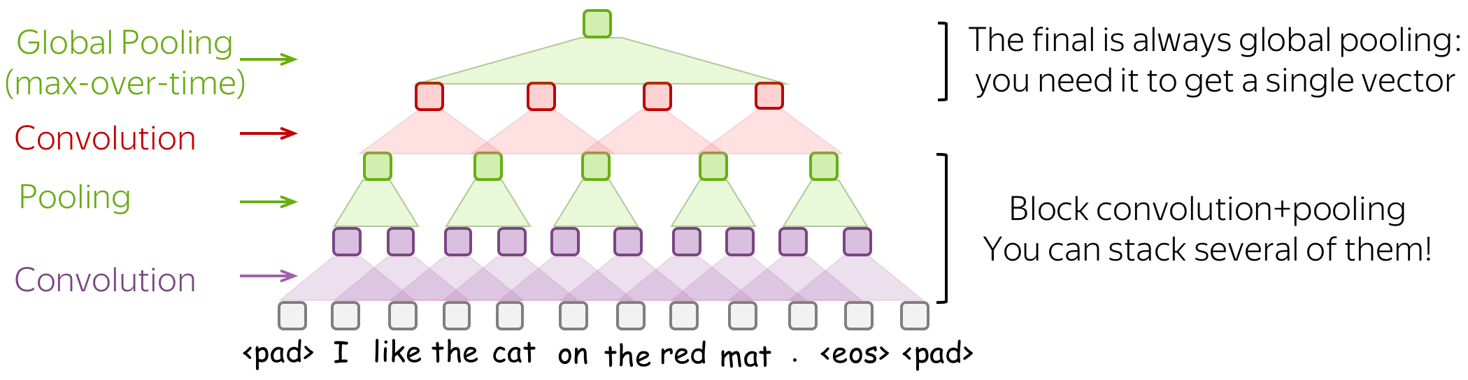
This idea was used, among others, in the paper Character-level Convolutional Networks for Text Classification.
Multi-Label Classification
Multi-label classification:
many labels, several can be correct
Multi-label classification:
many labels, several can be correct
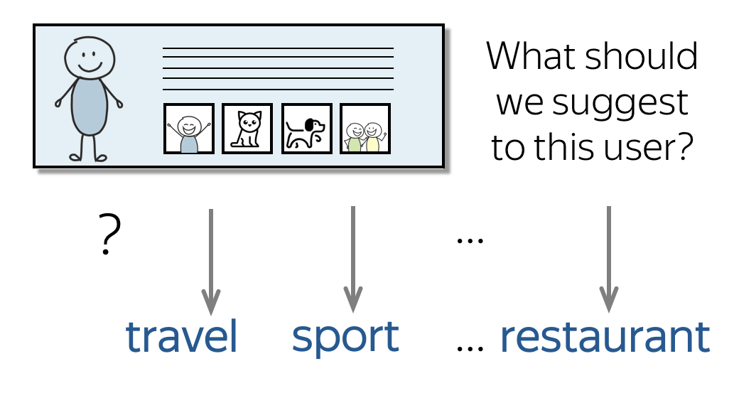
Multi-label classification is different from the single-label problems we discussed before in that each input can have several correct labels. For example, a twit can have several hashtags, a user can have several topics of interest, etc.
For a multi-label problem, we need to change two things in the single-label pipeline we discussed before:
- model (how we evaluate class probabilities);
- loss function.
Model: Softmax → Element-wise Sigmoid
After the last linear layer, we have \(K\) values corresponding to the \(K\) classes - these are the values we have to convert to class probabilities.
For single-label problems, we used softmax: it converts \(K\) values into a probability distribution, i.e. sum of all probabilities is 1. It means that the classes share the same probability mass: if the probability of one class is high, other classes can not have large probability (Lena: Once again, imagine a bunch of kittens eating from the same bowl: one kitten always eats at the expense of the others).
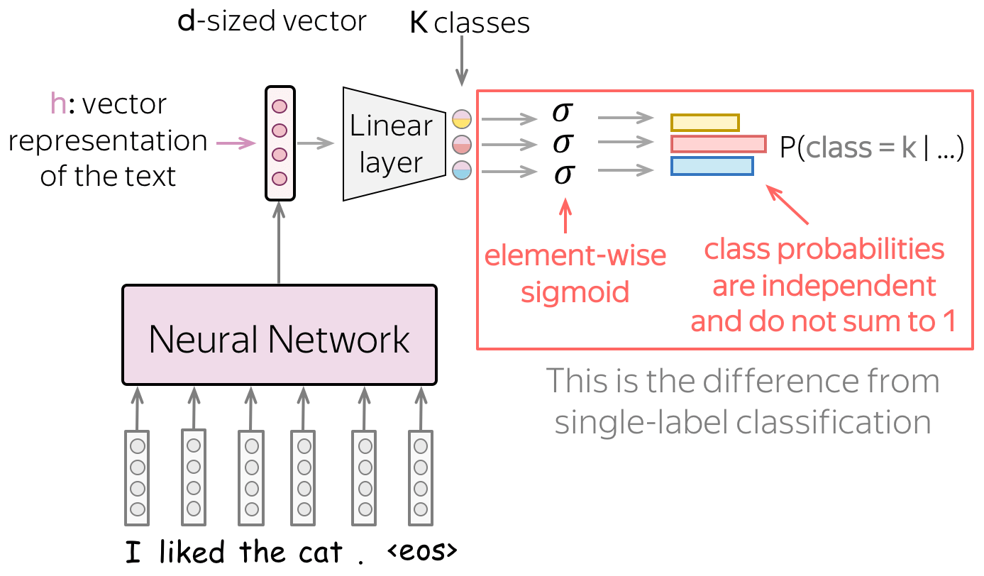
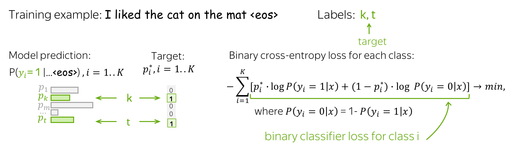
For multi-label problems, we convert each of the \(K\) values into a probability of the corresponding class independently from the others. Specifically, we apply the sigmoid function \(\sigma(x)=\frac{1}{1+e^{-x}}\) to each of the \(K\) values.
Intuitively, we can think of this as having \(K\) independent binary classifiers that use the same text representation.
Loss Function: Binary Cross-Entropy for Each Class
Loss function changes to enable multiple labels: for each class, we use the binary cross-entropy loss. Look at the illustration.
Practical Tips
Word Embeddings: how to deal with them?
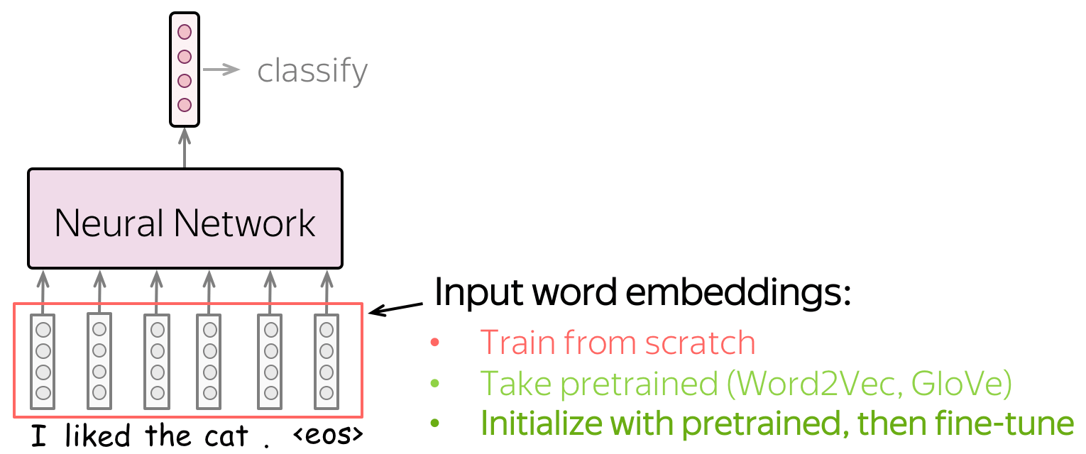
Input for a network is represented by word embeddings. You have three options how to get these embeddings for your model:
- train from scratch as part of your model,
- take pretrained (Word2Vec, GloVe, etc) and fix them (use them as static vectors),
- initialize with pretrained embeddings and train them with the network ("fine-tune").
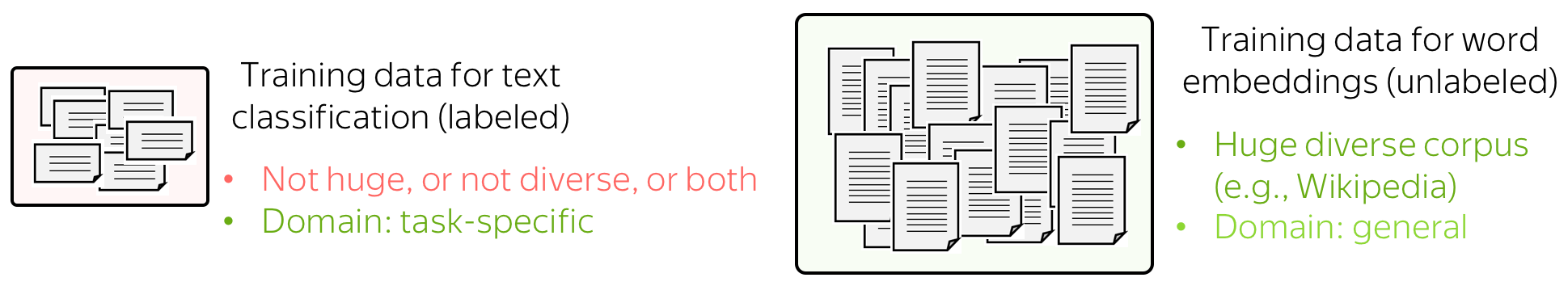
Let's think about these options by looking at the data a model can use. Training data for classification is labeled and task-specific, but labeled data is usually hard to get. Therefore, this corpus is likely to be not huge (at the very least), or not diverse, or both. On the contrary, training data for word embeddings is not labeled - plain texts are enough. Therefore, these datasets can be huge and diverse - a lot to learn from.
Now let us think what a model will know depending on what we do with the embeddings. If the embeddings are trained from scratch, the model will "know" only the classification data - this may not be enough to learn relationships between words well. But if we use pretrained embeddings, they (and, therefore, the whole model) will know a huge corpus - they will learn a lot about the world. To adapt these embeddings to your task-specific data, you can fine-tune these embeddings by training them with the whole network - this can bring gains in the performance (not huge though).
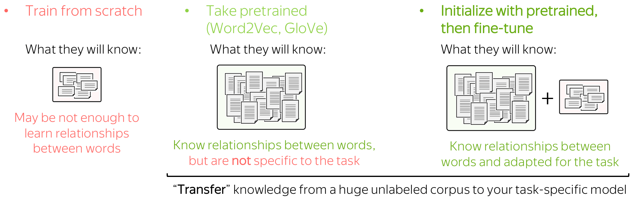
When we use pretrained embeddings, this is an example of transfer learning: through the embeddings, we "transfer" the knowledge of their training data to our task-specific model. We will learn more about transfer learning later in the course.
Fine-tune pretrained embeddings or not? Before training models, you can first think
why fine-tuning can be useful, and which types of examples can benefit from it.
Learn more from this exercise
in the Research Thinking section.
For more details and the experiments with different settings for word embeddings, look at this paper summary.
Data Augmentation: Get More Data for Free
Data augmentation alters your dataset in different ways to get alternative versions of the same training example. Data augmentation can increase
- the amount of data
Quality of your model depends a lot on your data. For deep learning models, having large datasets is very (very!) important. - diversity of data
By giving different versions of training examples, you teach a model to be more robust to real-world data which can be of lower quality or simply a bit different from your training data. With augmented data, a model is less likely to overfit to specific types of training examples and will rely more on general patterns.
Data augmentation for images can be done easily: look at the examples below. The standard augmentations include flipping an image, geometrical transformations (e.g. rotation and stretching along some direction), covering parts of an image with different patches.
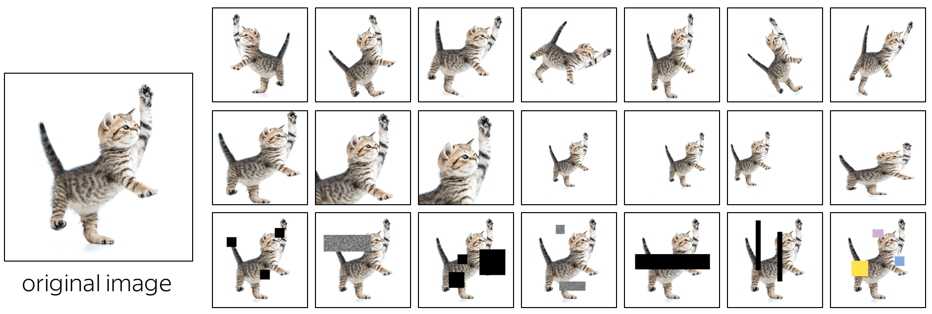
How can we do something similar for texts?
• word dropout - the most simple and popular
Word dropout is the simplest regularization: for each example, you choose some words randomly (say, each word is chosen with probability 10%) and replace the chosen words with either the special token UNK or with a random token from the vocabulary.
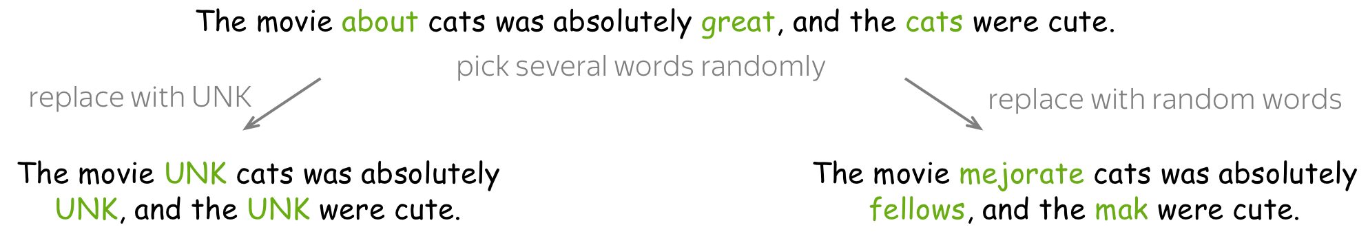
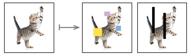
The motivation here is simple: we teach a model not to over-rely on individual tokens, but take into consideration context of the whole text. For example, here we masked great, and a model has to understand the sentiment based on other words.
Note: For images, this corresponds to masking out some areas. By masking out an area of an image, we also want a model not to over-rely on local features and to make use of a more global context.
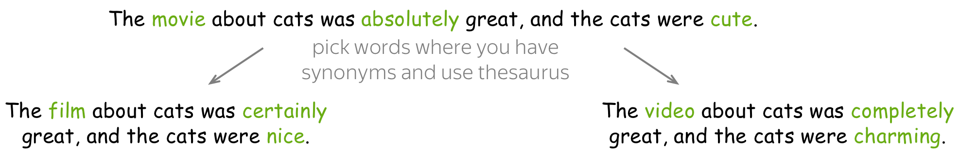
• use external resources (e.g., thesaurus) - a bit more complicated
A bit more complicated approach is to replace words or phrases with their synonyms. The tricky part is getting these synonyms: you need external resources, and they are rarely available for languages other than English (for English, you can use e.g. WordNet). Another problem is that for languages with rich morphology (e.g., Russian) you are likely to violate the grammatical agreement.
• use separate models - even more complicated
An even more complicated method is to paraphrase the whole sentences using external models. A popular paraphrasing method is to translate a sentence to some language and back. We will learn how to train a translation model a bit later (in the Seq2seq and Attention lecture), but for now, you can use industrial systems, e.g. Yandex Translate, Google Translate, etc. (Lena: Obviously, personally I'm biased towards Yandex :) ) Note that you can combine translation systems and languages to get several paraphrases.
Note: For images, the last two techniques correspond to geometric transformations: we want to change text, but to preserve the meaning. This is different from word dropout, where some parts are lost completely.
Analysis and Interpretability
What do Convolutions Learn? Analyzing Convolutional Filters
Convolutions in Computer Vision: Visual Patterns
Convolutions were originally developed for images, and there's already a pretty good understanding of what the filters capture and how filters from different layers from a hierarchy. While lower layers capture simple visual patterns such as lines or circles, final layers can capture the whole pictures, animals, people, etc.
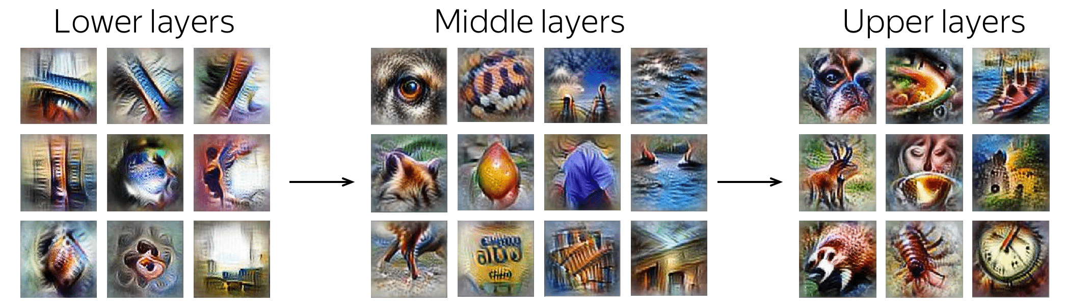
Examples of patterns captured by convolution filters for images.
The examples are from
Activation Atlas from distill.pub.
What About Convolutions in Texts?
This part is based on the paper Understanding Convolutional Neural Networks for Text Classification.
For images, filters capture local visual patterns which are important for classification. For text, such local patterns are word n-grams. The main findings on how CNNs work for texts are:
- convolving filters are used as ngram detectors
Each filter specializes in one or several families of closely-related ngrams. Filters are not homogeneous, i.e. a single filter can, and often does, detect multiple distinctly different families of ngrams. - max-pooling induces a thresholding behavior
Values below a given threshold are ignored when (i.e. irrelevant to) making a prediction. For example, this paper shows that 40% of the pooled ngrams on average can be dropped with no loss of performance.
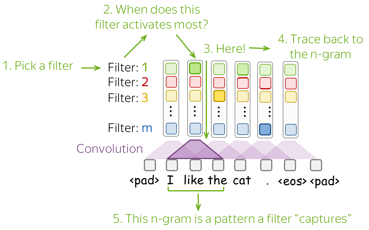
The simplest way to understand what a network captures is to look which patterns activate its neurons. For convolutions, we pick a filter and find those n-grams which activate this filter most.
Below are examples of the top-1 n-gram for several filters. For one of them, we also show other n-grams which lead to high activation of this filter - you can see that the n-grams have a very similar meaning.
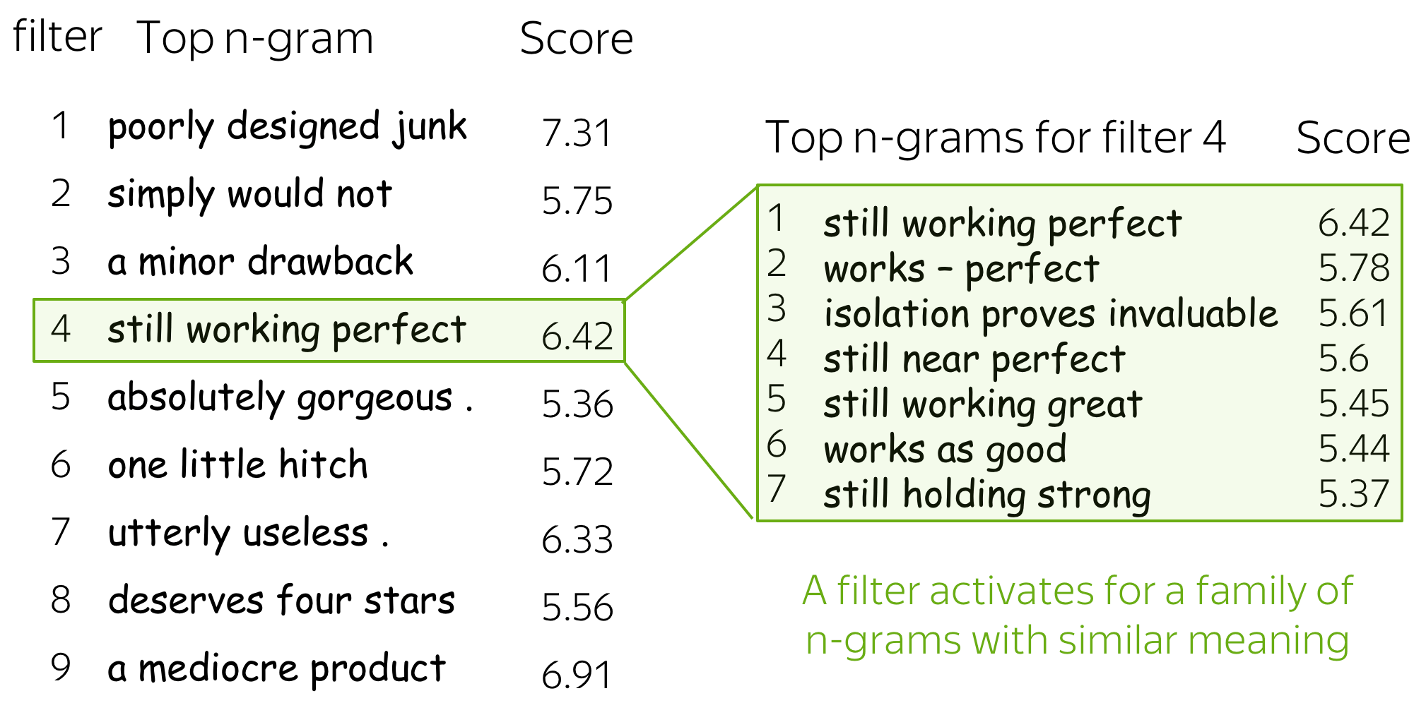
For more details, look at the paper Understanding Convolutional Neural Networks for Text Classification.
How About RNN CLassifiers?
How RNNs trained for classification process text? Learn here.
Research Thinking
Classical Approaches
The simplest Naive Bayes implementation uses tokens as features. However, this is not always good: completely different texts can have the same features.
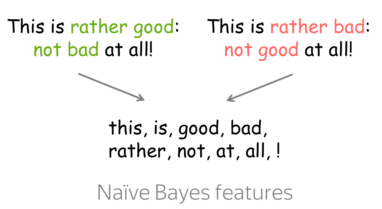
Possible answers
Idea: Add Frequent N-Grams to the Features!
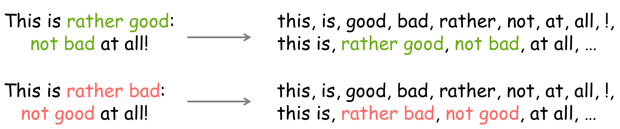
Instead of using only words as features, we can also use word n-grams. Since using all n-grams would be inefficient, we can add only the frequent ones. This can fix some examples with simple negation as the one shown above.
? What other types of features you can come up with?
Possible answers
Note that Naive Bayes can use any categorical features - you can do anything as long as you can compute the counts for probabilities. For example,
- text length
Who knows - maybe positive reviews are longer than negative? Don't forget to categorize it, e.g., 1-20 tokens correspond to one feature, 21-30 tokens - to another, etc. - token frequency
It may be worth checking - positive or negative reviews use more peculiar words? You can come up with some characteristics of tokens frequency: minimum of maximum, average, etc. But again - you have to categorize it! - syntactical features
(if you don't know what it is yet, skip this)
Dependency tree depth (maximum/minimum/average) - this can be a proxy of text complexity. - anything else you can come up with
Just try :)
? Are all words equally needed for classification? If not, how can we modify the method?
Possible answers
Idea: Do Not Use Unimportant Words
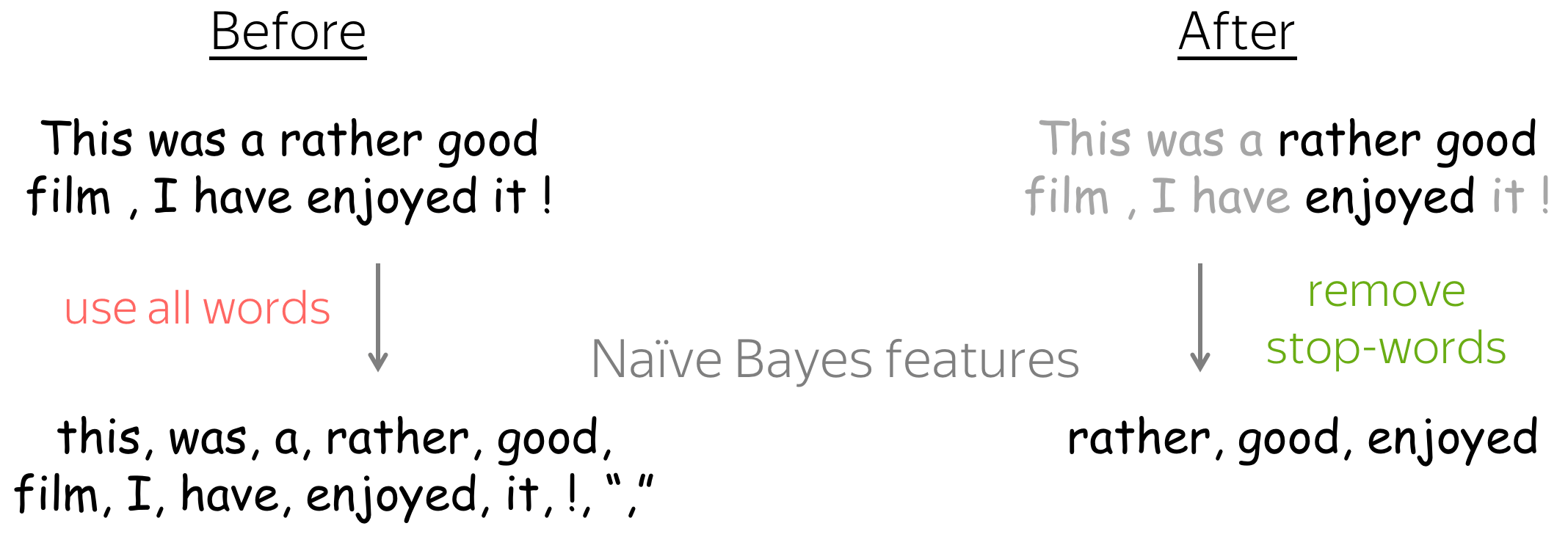
If you know which words definitely do not influence class probability, you can remove them from the features! For example, we can remove stop-words: determiners, prepositions, etc.
Note: you need to be really careful - don't remove something useful!
Neural Approaches
Before training models, you can first think why fine-tuning can be useful, and which types of examples can benefit from it. Remember how embeddings are trained: words that are used similarly in texts have very close embeddings. Therefore, sometimes antonyms are closest to each other, e.g. descent and ascent.
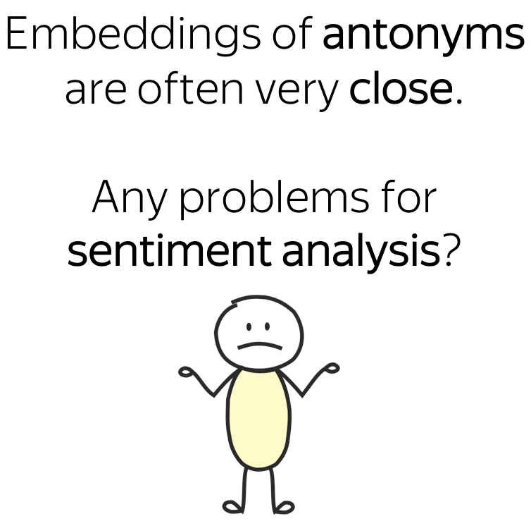
Possible answers
Without fine-tuning, closest to bad is good!
The figure shows closest neighbors of Word2Vec embeddings before and after fine-tuning (examples are taken from this paper).
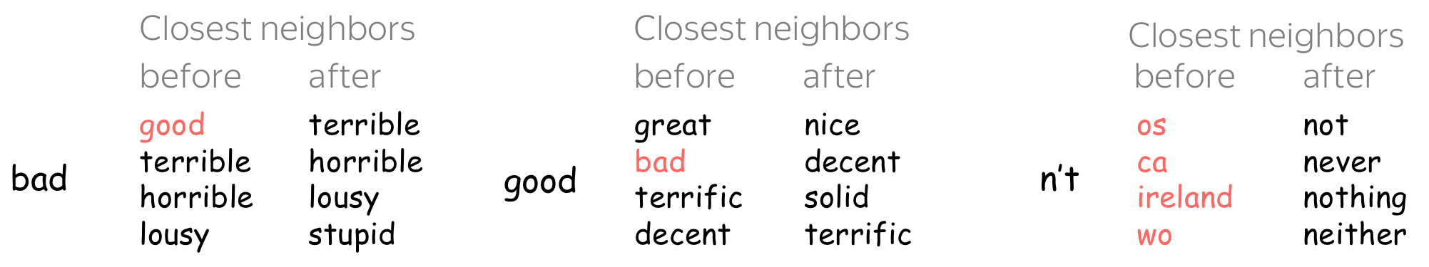
Without fine-tuning, closest to bad is good! Without fine-tuning, it would be very hard for a model to separate positive and negative using these embeddings. This is only one example of antonyms with close embeddings which can hurt sentiment classification.
Fine-tuning can also help to improve understanding of tokens such as n't: rare in the corpus word embeddings were trained on, but not rare in the corpus we care about. More generally, if your task-specific domain is different from the word embeddings training data, fine-tuning is a good idea.
Here will be more exercises!
This part will be expanding from time to time.

Related Papers
What's inside:
- Convolutions for Classification: Classics
- Analyzing RNNs for Sentiment Classification
- ... to be updated
Convolutions for Classification: Classics
Even a very simple CNN with one layer on top of word embeddings shows very good performance (without features requiring some external knowledge!). The paper also shows the importance of using pretrained embeddings (and not training from scratch) and gains from fine-tuning.
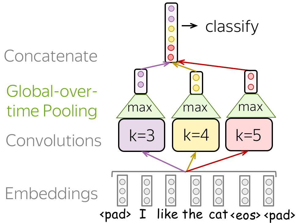
More details
The CNN model is shown on the figure: on top of embeddings, it has three convolutions with max-over-time pooling (in parallel). The results are concatenated and used for classification. This is a very simple model we discussed earlier.
The paper has a lot of results (comparison with 14 baselines!), but here I'll mention only the ones comparing the same CNN model with different strategies of obtaining word embeddings.
Embeddings: Random vs Pretrained (Word2Vec)
In the table below random experiment - embeddings are randomly initialized and trained with the model, pretrained - the embeddings are initialized with Word2Vec and fixed (not trained with the model).
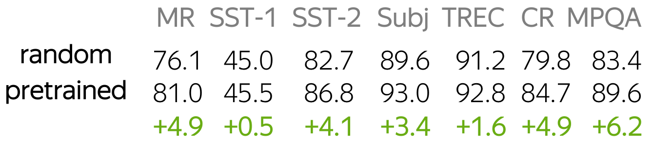
We see that using pretrained embeddings is better by several percentage points! This happens because in the first case the embeddings see only the classification training data, which is usually not much. But trained embeddings saw a lot of other data - they know a lot more about the world and relationships between words.
Important! This is called transfer learning - by using trained embeddings, you "transfer" knowledge contained in the embeddings training data to your model. We will learn more about this later in the course.
Pretrained Embeddings: Fixed vs Fine-tuned
In the table below fixed experiment - the embeddings are initialized with Word2Vec and fixed (not trained with the model), fine-tuned - the embeddings are initialized with Word2Vec and then trained with the classification model.
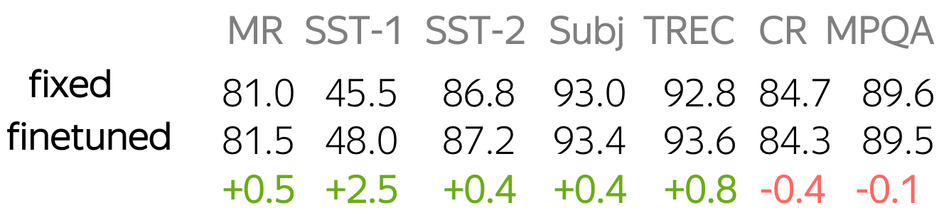
We see that if we fine-tune pretrained embeddings for the specific task, we are likely to get further improvement. But you need to be careful - embeddings can "forget" what they learned before.
More in the paper
- comparison with lots of baselines
This simple model performs quite well compared to lots of baselines (including SVMs we discussed above). - both fixed and fine-tuned embeddings
The paper proposes a way to use both fixed embeddings and fine-tuned: it duplicates the embedding layer and keeps one of them fixed while trains the other. The results are mixed - look in the paper!
This is the first paper showing that CNNs only on characters can do quite well. This is interesting: classification can be done without any external knowledge, even without text segmentation into words! An important point is that character-level CNNs can do better than classical approaches only for large datasets.
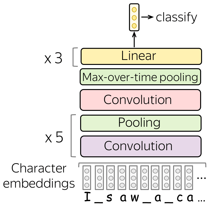
More details
The CNN model is shown in the figure above. It has 6 convolution+pooling blocks (note that the last pooling is global) followed by 3 linear layers (with non-linearities after each convolution and linear layers).
Character-level CNN is better for large datasets
The figure below shows the relative errors with respect to comparison models. Each of these plots is computed by taking the difference between errors on a comparison model and the character-level CNN model, then divided by the comparison model error.
Here we show only 2 of the comparisons: with a classical approach (n-grams tf-idf) and a word-level CNN. The results show that for large datasets, character-level CNN performs better.
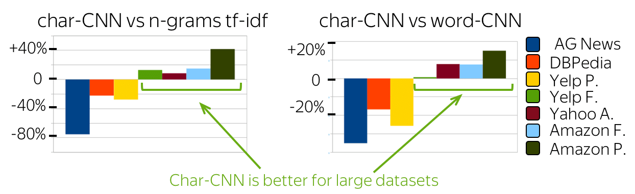
Other Results
- choice of alphabet matters
You can take either only lowercased data, or distinguish between uppercase and lowercase - the results can be different! - char-CNNs work better for user-generated data.
Compared to word-level models, character-level ones may be better suitable for raw user data with misspellings.
For more details, look at the paper!
Analyzing RNNs for Sentiment Classification
If we take an RNN trained for sentiment analysis and apply PCA to lots of its states, we'll see that almost all variance is explained with only two components. Moreover, when such RNN reads a text, its states move along a 1D plane in either negative or positive direction depending on the word it reads.
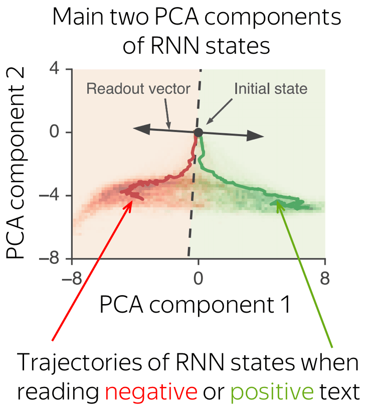
More details
The paper looks at four different RNN types (vanilla, LSTM, GRU, and the Update Gate RNN), as well as different sentiment classification datasets (IMDb movie review, Yelp review, SST-2). The results are similar for all combinations.
PCA: Most of the Variance is Captured by a Few Dimensions
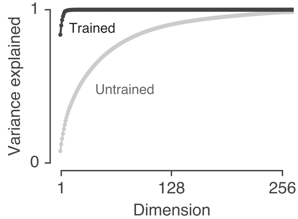
The authors took 1000 test examples, fed it to LSTM, took all states, and applied PCA. Turns out, all variance is explained by only a couple of components! Note that this is true only for a trained model - for untrained one, this is not the case. Look at the figure.
The 1D Plane, Trajectories and Word Influences
In the figure above (the red/green one) are the RNN states projected onto the first two PCA components; the states are colored according to the target label. We see that the states lie along a one-dimensional plane corresponding to the sentiment changing from one to another. The figure also shows examples of RNN trajectories when reading a positive or a negative text. The further the model is in the text, the deeper its state goes in the corresponding area.
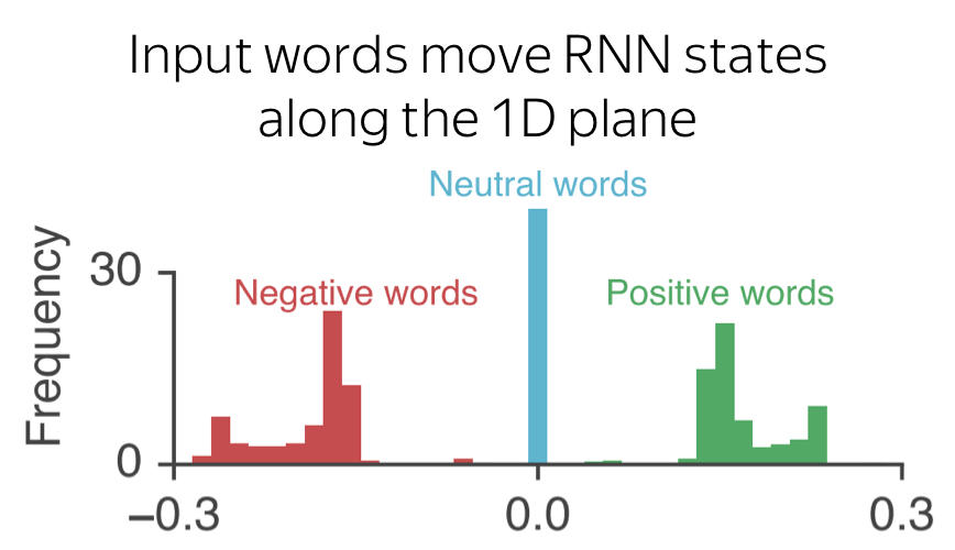
What is more interesting, the authors also looked at how each token influences the RNN state. As expected, positive and negative words usually move the states in the corresponding area, while neutral words do not have such influence.
More in the paper
- linear approximations of RNN dynamics
The authors apply a linearization procedure to obtain an approximate, but highly interpretable, description of the RNN dynamics. - RNNs count the number of positive and negative words used
With lots of math, the authors conclude that in nearly all cases the key activity performed by the RNN for sentiment analysis is simply counting the number of positive and negative words used.
Here will be more papers!
The papers will be gradually appearing.

Have Fun!
Coming soon!
We are still working on this!