Language Modeling
What does it mean to "model something"?
Imagine that we have, for example, a model of a physical world. What do you expect it to be able to do? Well, if it is a good model, it probably can predict what happens next given some description of "context", i.e., the current state of things. Something of the following kind:
We have a tower of that many toy cubes of that size made from this material. We push the bottom cube from this point in that direction with this force. What will happen?
A good model would simulate the behavior of the real world: it would "understand" which events are in better agreement with the world, i.e., which of them are more likely.
What about language?
For language, the intuition is exactly the same! What is different, is the notion of an event. In language, an event is a linguistic unit (text, sentence, token, symbol), and a goal of a language model is to estimate the probabilities of these events.
Language Models (LMs) estimate the probability of different linguistic units: symbols, tokens, token sequences.
But how can this be useful?
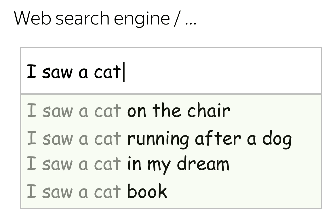
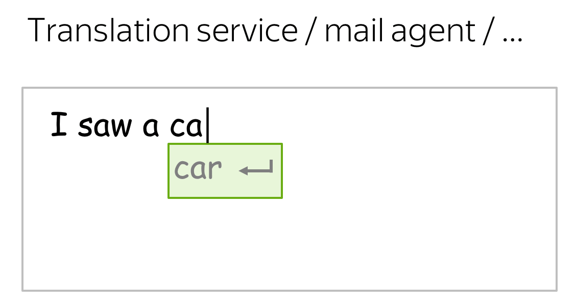
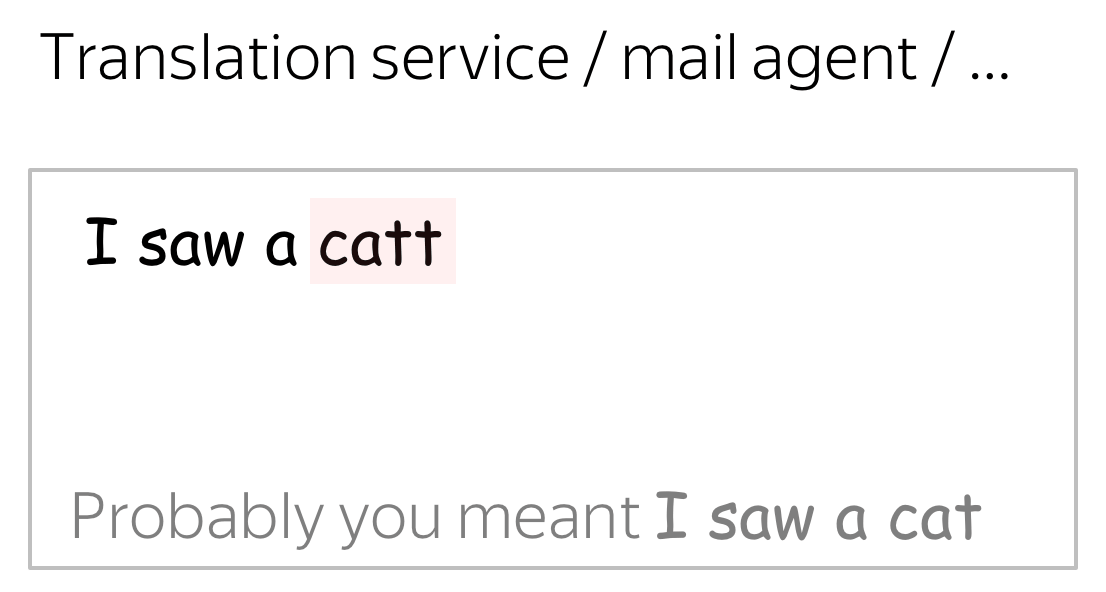
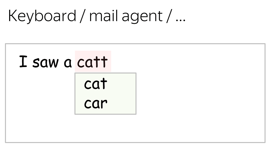
We deal with LMs every day!
We see language models in action every day - look at some examples. Usually models in large commercial services are a bit more complicated than the ones we will discuss today, but the idea is the same: if we can estimate probabilities of words/sentences/etc, we can use them in various, sometimes even unexpected, ways.
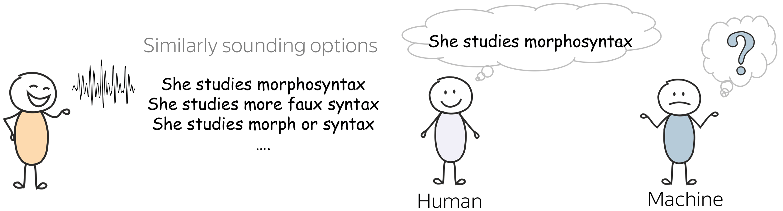
What is easy for humans, can be very hard for machines
Foundations of Natural Language Processing course at the University of Edinburgh.
We, humans, already have some feeling of "probability" when it comes to natural language. For example, when we talk, usually we understand each other quite well (at least, what's being said). We disambiguate between different options which sound similar without even realizing it!
But how a machine is supposed to understand this? A machine needs a language model, which estimates the probabilities of sentences. If a language model is good, it will assign a larger probability to a correct option.
General Framework
Text Probability
Our goal is to estimate probabilities of text fragments; for simplicity, let's assume we deal with sentences. We want these probabilities to reflect knowledge of a language. Specifically, we want sentences that are "more likely" to appear in a language to have a larger probability according to our language model.
How likely is a sentence to appear in a language?
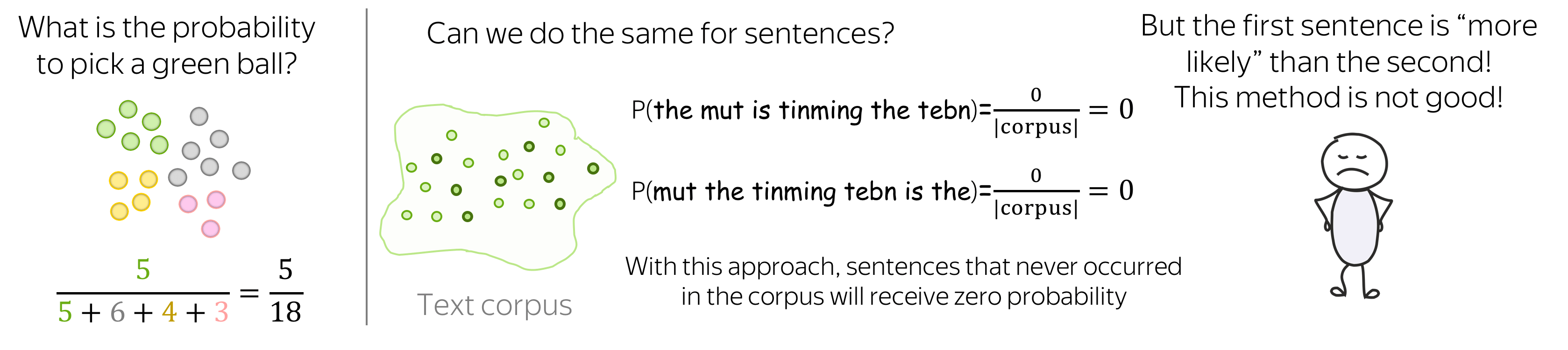
Let's check if simple probability theory can help. Imagine we have a basket with balls of different colors. The probability to pick a ball of a certain color (let's say green) from this basket is the frequency with which green balls occur in the basket.
What if we do the same for sentences? Since we can not possibly have a text corpus that contains all sentences in a natural language, a lot of sentences will not occur in the corpus. While among these sentences some are clearly more likely than the others, all of them will receive zero probability, i.e., will look equally bad for the model. This means, the method is not good and we have to do something more clever.
Sentence Probability: Decompose Into Smaller Parts
We can not reliably estimate sentence probabilities if we treat them as atomic units. Instead, let's decompose the probability of a sentence into probabilities of smaller parts.
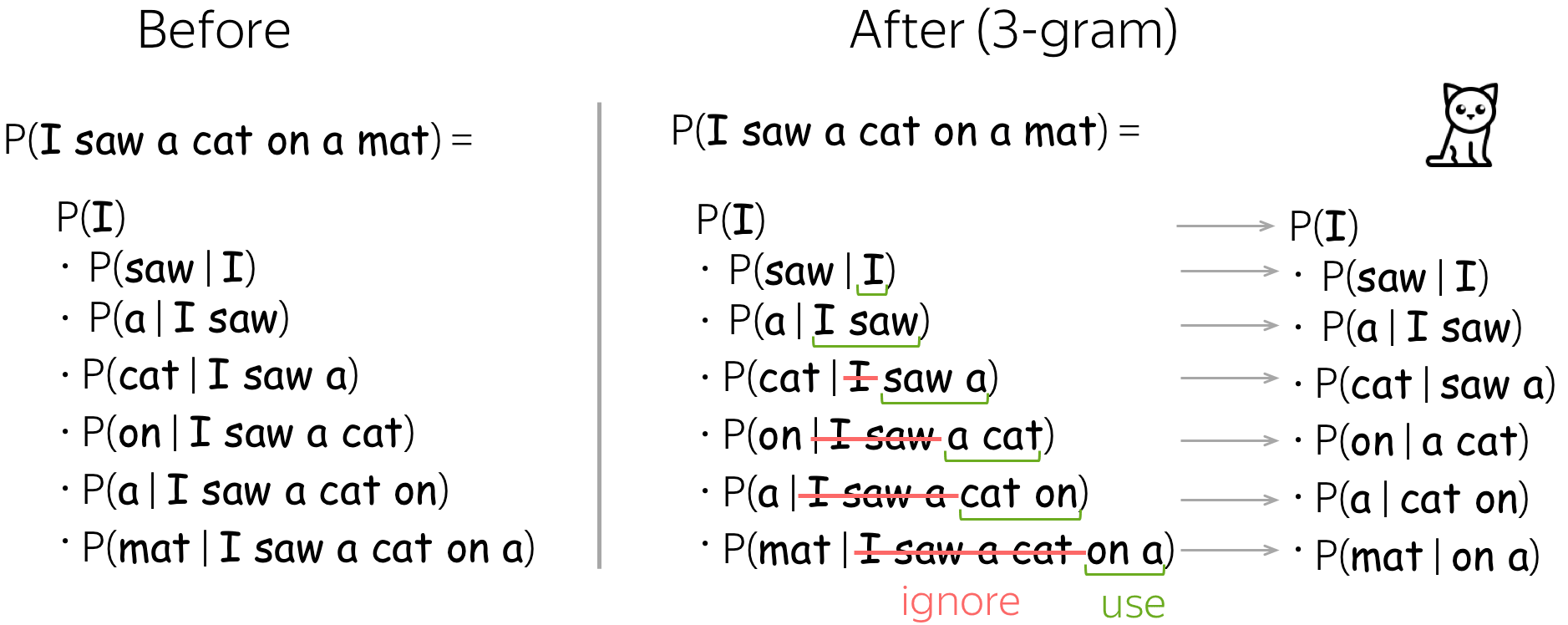
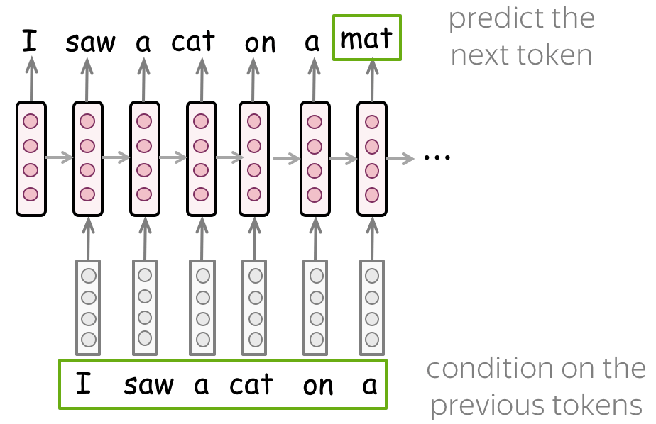
For example, let's take the sentence I saw a cat on a mat and imagine that we read it word by word. At each step, we estimate the probability of all seen so far tokens. We don't want any computations not to be in vain (no way!), so we won't throw away previous probability once a new word appears: we will update it to account for a new word. Look at the illustration.

Formally, let \(y_1, y_2, \dots, y_n\) be tokens in a sentence, and \(P(y_1, y_2, \dots, y_n)\) the probability to see all these tokens (in this order). Using the product rule of probability (aka the chain rule), we get \[P(y_1, y_2, \dots, y_n)=P(y_1)\cdot P(y_2|y_1)\cdot P(y_3|y_1, y_2)\cdot\dots\cdot P(y_n|y_1, \dots, y_{n-1})= \prod \limits_{t=1}^n P(y_t|y_{\mbox{<}t}).\] We decomposed the probability of a text into conditional probabilities of each token given the previous context.
We got: Left-to-Right Language Models
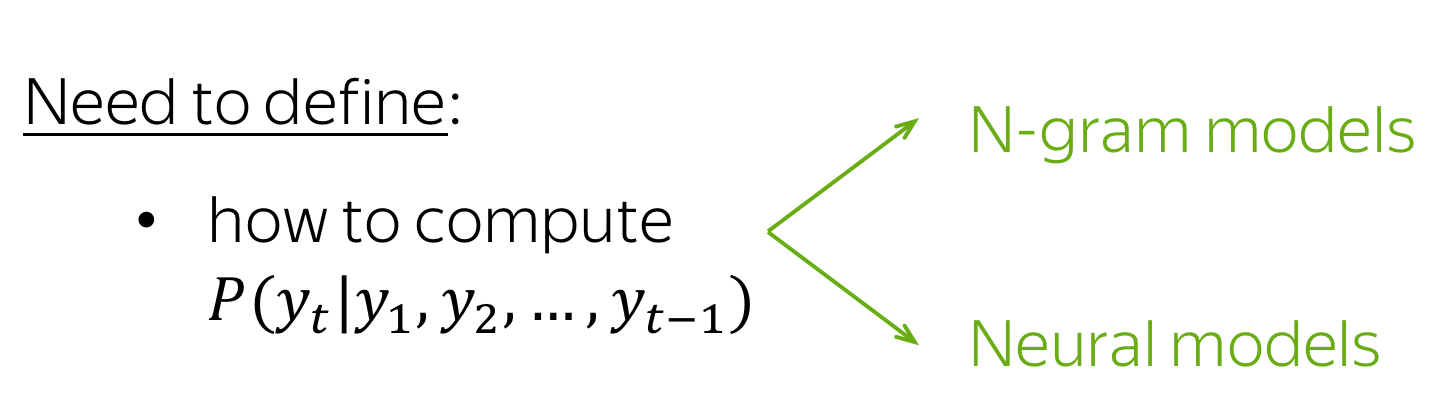
What we got is the standard left-to-right language modeling framework. This framework is quite general: N-gram and neural language models differ only in a way they compute the conditional probabilities \(P(y_t|y_1, \dots, y_{t-1})\).
Lena: Later in the course we will see other language models: for example, Masked Language Models or models that decompose the joint probability differently (e.g., arbitrary order of tokens and not fixed as the left-to-right order).
We will come to specifics of N-gram and neural models a bit later. Now, we discuss how to generate a text using a language model.
Generate a Text Using a Language Model
Once we have a language model, we can use it to generate text. We do it one token at a time: predict the probability distribution of the next token given previous context, and sample from this distribution.
Alternatively, you can apply greedy decoding: at each step, pick the token with the highest probability. However, this usually does not work well: a bit later I will show you examples from real models.
Despite its simplicity, such sampling is quite common in generation. In section Generation Strategies we will look at different modifications of this approach to get samples with certain qualities; e.g., more or less "surprising".
N-gram Language Models
Let us recall that the general left-to-right language modeling framework decomposes probability of a token sequence, into conditional probabilities of each token given previous context: \[P(y_1, y_2, \dots, y_n)=P(y_1)\cdot P(y_2|y_1)\cdot P(y_3|y_1, y_2)\cdot\dots\cdot P(y_n|y_1, \dots, y_{n-1})= \prod \limits_{t=1}^n P(y_t|y_{\mbox{<}t}).\] The only thing which is not clear so far is how to compute these probabilities.
We need to: define how to compute the conditional probabilities \(P(y_t|y_1, \dots, y_{t-1})\).
Similar to count-based methods we saw earlier in the Word Embeddings lecture, n-gram language models also count global statistics from a text corpus.
How: estimate based on global statistics from a text corpora, i.e., count.
That is, the way n-gram LMs estimate probabilities \(P(y_t|y_{\mbox{<}t}) = P(y_t|y_1, \dots, y_{t-1})\) is almost the same as the way we earlier estimated the probability to pick a green ball from a basket. This innocent "almost" contains the key components of n-gram LMs: Markov property and smoothings.
Markov Property (Independence Assumption)
The straightforward way to compute \(P(y_t|y_1, \dots, y_{t-1})\) is \[P(y_t|y_1, \dots, y_{t-1}) = \frac{N(y_1, \dots, y_{t-1}, y_t)}{N(y_1, \dots, y_{t-1})},\] where \(N(y_1, \dots, y_k)\) is the number of times a sequence of tokens \((y_1, \dots, y_k)\) occur in the text.
For the same reasons we discussed before, this won't work well: many of the fragments \((y_1, \dots, y_{t})\) do not occur in a corpus and, therefore, will zero out the probability of the sentence. To overcome this problem, we make an independence assumption (assume that the Markov property holds):
The probability of a word only depends on a fixed number of previous words.
- n=3 (trigram model): \(P(y_t|y_1, \dots, y_{t-1}) = P(y_t|y_{t-2}, y_{t-1})\),
- n=2 (bigram model): \(P(y_t|y_1, \dots, y_{t-1}) = P(y_t|y_{t-1})\),
- n=1 (unigram model): \(P(y_t|y_1, \dots, y_{t-1}) = P(y_t)\).
Look how the standard decomposition changes for n-gram models.
Smoothing: Redistribute Probability Mass
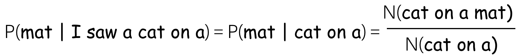
Let's imagine we deal with a 4-gram language model and consider the following example:
What if either denominator or numerator is zero? Both these cases are not really good for the model. To avoid these problems (and some other), it is common to use smoothings. Smoothings redistribute probability mass: they "steal" some mass from seen events and give to the unseen ones.
Lena: at this point, usually I'm tempted to imagine a brave Robin Hood, stealing from the rich and giving to the poor - just like smoothings do with the probability mass. Unfortunately, I have to stop myself, because, let's be honest, smoothings are not so clever - it would be offensive to Robin.
Avoid zeros in the denominator
If the phrase cat on a never appeared in our corpus, we will not be able to compute the probability. Therefore, we need a "plan B" in case this happens.
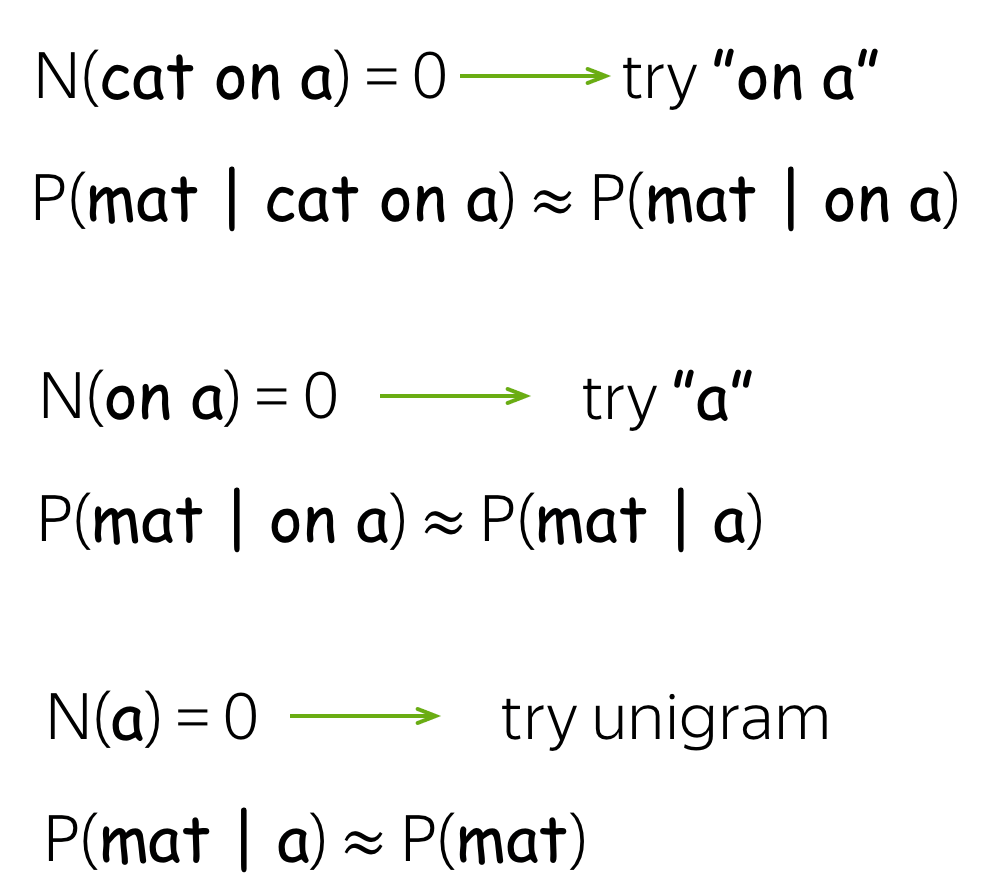
Backoff (aka Stupid Backoff)
One of the solutions is to use less context for context we don't know much about. This is called backoff:
- if you can, use trigram;
- if not, use bigram;
- if even bigram does not help, use unigram.
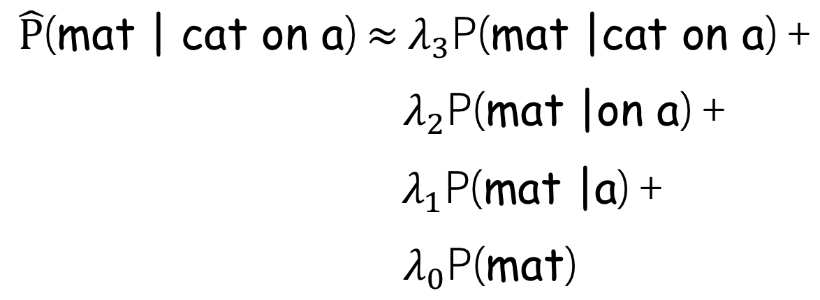
More clever: Linear interpolation
A more clever solution is to mix all probabilities: unigram, bigram, trigram, etc. For this, we need scalar positive weights \(\lambda_0, \lambda_1, \dots, \lambda_{n-1}\) such that \(\sum\limits_{i}\lambda_i=1\). Then the updated probability is:
Avoid zeros in the numerator
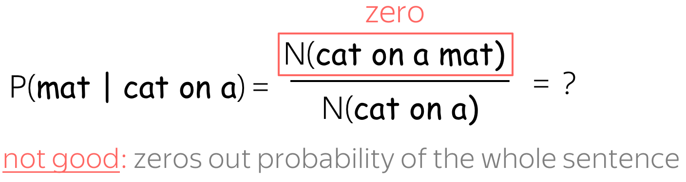
If the phrase cat on a mat never appeared in our corpus, the probability of the whole sentence will be zero - but this does not mean that the sentence is impossible! To avoid this, we also need a "plan B".
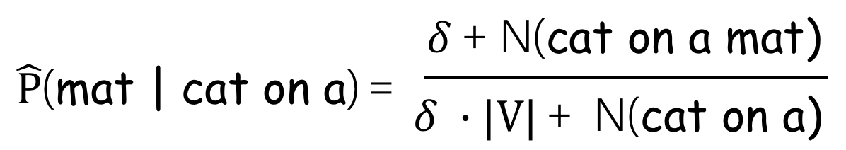
Laplace smoothing (aka add-one smoothing)
The simplest way to avoid this is just to pretend we saw all n-grams at least one time: just add 1 to all counts! Alternatively, instead of 1, you can add a small \(\delta\):
More Clever Smoothings
Kneser-Ney Smoothing.
The most popular smoothing for n-gram LMs is Kneser-Ney smoothing:
it is a more clever variant of the back-off.
More details are here.
Generation (and Examples)
The generation procedure for a n-gram language model is the same as the general one: given current context (history), generate a probability distribution for the next token (over all tokens in the vocabulary), sample a token, add this token to the sequence, and repeat all steps again. The only part which is specific to n-gram models is the way we compute the probabilities. Look at the illustration.
Examples of generated text
To show you some examples, we trained a 3-gram model on 2.5 million English sentences.
Dataset details.
The data is the English
side of WMT English-Russian translation data. It consists of 2.5 million sentence pairs
(a pair of sentences in English and Russian which are supposed to be translations of each other).
The dataset
contains news data, Wikipedia titles and 1 million crawled sentences released by Yandex.
This data is one of the standard datasets for machine translation; for language modeling,
we used only the English side.
Note that everything you will see below is generated by a model and presented
without changes or filtering. Any content you might not like
appeared as a result of training data. The best we can do is to use the standard datasets, and we did.
How to: Look at the samples from a n-gram LM. What is clearly wrong with these samples? What in the design of n-gram models leads to this problem?
so even when i talk a bit short , there was no easy thing to do different buffer flushing strategies in the future , due to huge list of number - one just has started production of frits in the process and has free wi - fi ” operation .... _eos_
he can perform the dual monarchy arrived in moscow lying at two workshops one in all schools of political science ..." and then you can also benefit from your service . _eos_
alas , still in the lower left corner will not start in 1989 . _eos_
john holmes is a crystal - clear spring of 2001 . _eos_
it simply yields a much later , there were present , ferrocenecontaining compounds for clinical trials in connection with this chapter you ' re looking for ways of payment and insert preferred record into catalogue of negative influences - military . _eos_
impotence in the way gazprom and its environment . _eos_
according to the address and tin box , luggage storage , gay friendly , all of europe to code - transitions . _eos_
26 . 01 page 2 introduction the challenge for the horizontal scroll bar in sweden , austria _eos_
the rza lyrics are brought to you , there are a few . _eos_
golden sands , once again the only non - governmental organizations recognized by the objector . _eos_
hahn , director of the christian " love and compassion " was designed as a result of any form , in the transaction is active in the stuva grill . _eos_
there is a master ’ s a major bus routes in and the us became israel were rewarded with an electric air conditioning television satellite television . _eos_
, we have had , 1990 in aksaray – turkey has provided application is built on low - power plants . _eos_
when this option may be the worst day of amnesty international delegations visited israel , and felt that his sisters , that they are reserved for zyryanovsk concentrating factory there is a member of the shire ," given as to damage the expansion of a meeting over a large health maintenance organization , smoking , airconditioning , designated smoking area . _eos_
4 . 0 beta has been received the following initiatives in order to meet again in 1989 , and in the face of director of branch offices in odessa on time , the church of norway is an advertisement for the protection the d - 54673 , limousine , employee badges , etc ) downloading this icecat data - do can talk about israel as well as standard therapy of czech republic estonia greece france ireland israel italy jamaica japan jordan kazakhstan kenya kiribati kuwait kyrgyzstan lao people ' s closing of the task of mill - a fire that _eos_
one lesson the teacher ! _eos_
pupils from eastern europe , africa , saudi arabia ’ s church , yearn for such an open structure of tables several times on monday 14 september 2003 , his flesh when i was curious to know and also to find what they are constructed with a speeding arrow . _eos_
blackjack : six steps to resolve complex social adaptation of the room ' s polyclinics and to english . _eos_
this is the right nanny jobs easier for people to take part in the history of england has a large number of regional and city administration . _eos_
melody for the acquisition , provision or condition . _eos_
they have a proper map that force distant astronomical objects have been soaring among ukrainians - warriors ". _eos_
also now recognizing how interdependent they are successful in emulating poland ’ s satisfaction . _eos_
we tried to make lyrics as correct as possible , however if you have any corrections for abecedário da xuxa lyrics are brought to you by lyrics - keeper . _eos_
49 . 99 webmoney rub , 893 . 6 million euros . _eos_
You probably noticed that these samples are not fluent: it can be clearly seen that the model does not use long context, and relies only on a couple of tokens. The inability to use long contexts is the main shortcoming of n-gram models.
Now, we take the same model, but perform greedy decoding: at each step, we pick the token with the highest probability. We used 2-token prefixes from the examples of samples above (for each example, the prefix fed to the model is underlined).
How to: Look at the examples generated by the same model using greedy decoding. Do you like these texts? How would you describe them?
so even if the us , and the united states , the hotel is located in the list of songs , you can add them in our collection by this form . _eos_
he can be used to be a good idea to the keyword / phrase business intelligence development studio . _eos_
alas , the hotel is located in the list of songs , you can add them in our collection by this form . _eos_
john holmes _eos_
it simply , the hotel is located in the list of songs , you can add them in our collection by this form . _eos_
impotence in the list of songs , you can add them in our collection by this form . _eos_
according to the keyword / phrase business intelligence development studio . _eos_
26 . _eos_
the rza ( bobby digital ) is a very good . _eos_
golden sands resort . _eos_
hahn , of the world . _eos_
there is a very good . _eos_
, we a good idea to the keyword / phrase business intelligence development studio . _eos_
when this option is to be a good idea to the keyword / phrase business intelligence development studio . _eos_
4 . 5 % of the world . _eos_
one lesson from the city of the world . _eos_
pupils from the city of the world . _eos_
blackjack : six - party talks . _eos_
this is the most important thing is that the us , and the united states , the hotel is located in the list of songs , you can add them in our collection by this form . _eos_
melody for two years , the hotel is located in the list of songs , you can add them in our collection by this form . _eos_
they have been a member of the world . _eos_
also now possible to use the " find in page " function below . _eos_
we tried to make lyrics as correct as possible , however if you have any corrections for the first time in the list of songs , you can add them in our collection by this form . _eos_
49 . _eos_
We see that greedy texts are:
- shorter - the _eos_ token has high probability;
- very similar - many texts end up generating the same phrase.
To overcome the main flaw of n-gram LMs, fixed context size, we will now come to neural models. As we will see later, when longer contexts are used, greedy decoding is not so awful.
Neural Language Models
In our general left-to-right language modeling framework, the probability of a token sequence is: \[P(y_1, y_2, \dots, y_n)=P(y_1)\cdot P(y_2|y_1)\cdot P(y_3|y_1, y_2)\cdot\dots\cdot P(y_n|y_1, \dots, y_{n-1})= \prod \limits_{t=1}^n P(y_t|y_{\mbox{<}t}).\] Let us recall, again, what is left to do.
We need to: define how to compute the conditional probabilities \(P(y_t|y_1, \dots, y_{t-1})\).
Differently from n-gram models that define formulas based on global corpus statistics, neural models teach a network to predict these probabilities.
How: Train a neural network to predict them.
Intuitively, neural Language Models do two things:
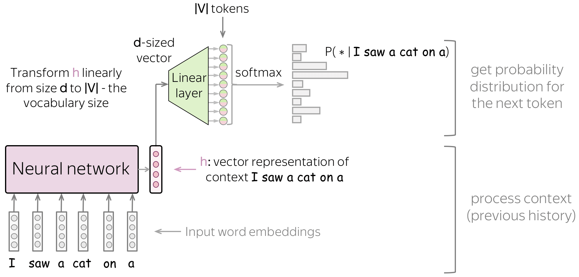
- process context → model-specific
The main idea here is to get a vector representation for the previous context. Using this representation, a model predicts a probability distribution for the next token. This part could be different depending on model architecture (e.g., RNN, CNN, whatever you want), but the main point is the same - to encode context. - generate a probability distribution for the next token → model-agnostic
Once a context has been encoded, usually the probability distribution is generated in the same way - see below.
This is classification!
We can think of neural language models as neural classifiers. They classify prefix of a text into |V| classes, where the classes are vocabulary tokens.
High-Level Pipeline
Since left-to-right neural language models can be thought of as classifiers, the general pipeline is very similar to what we saw in the Text Classification lecture. For different model architectures, the general pipeline is as follows:
- feed word embedding for previous (context) words into a network;
- get vector representation of context from the network;
- from this vector representation, predict a probability distribution for the next token.
Similarly to neural classifiers, we can think about the classification part (i.e., how to get token probabilities from a vector representation of a text) in a very simple way.
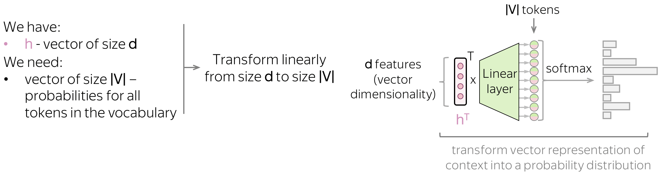
Vector representation of a text has some dimensionality \(d\), but in the end, we need a vector of size \(|V|\) (probabilities for \(|V|\) tokens/classes). To get a \(|V|\)-sized vector from a \(d\)-sized, we can use a linear layer. Once we have a \(|V|\)-sized vector, all is left is to apply the softmax operation to convert the raw numbers into class probabilities.
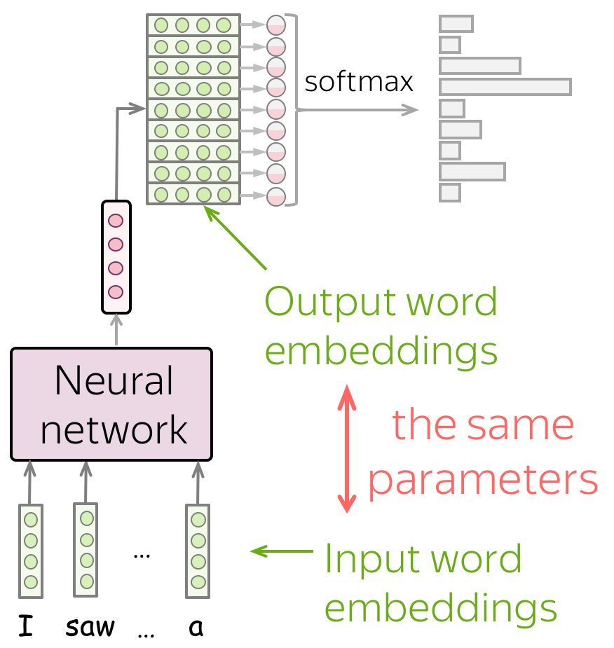
Another View: Dot Product with Output Word Embeddings
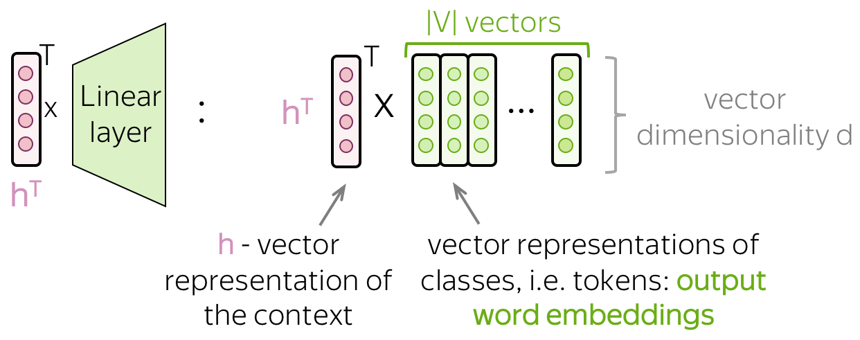
If we look at the final linear layer more closely, we will see that it has \(|V|\) columns and each of them corresponds to a token in the vocabulary. Therefore, these vectors can be thought of as output word embeddings.
Now we can change our model illustration according to this view. Applying the final linear layer is equivalent to evaluating the dot product between text representation h and each of the output word embeddings.
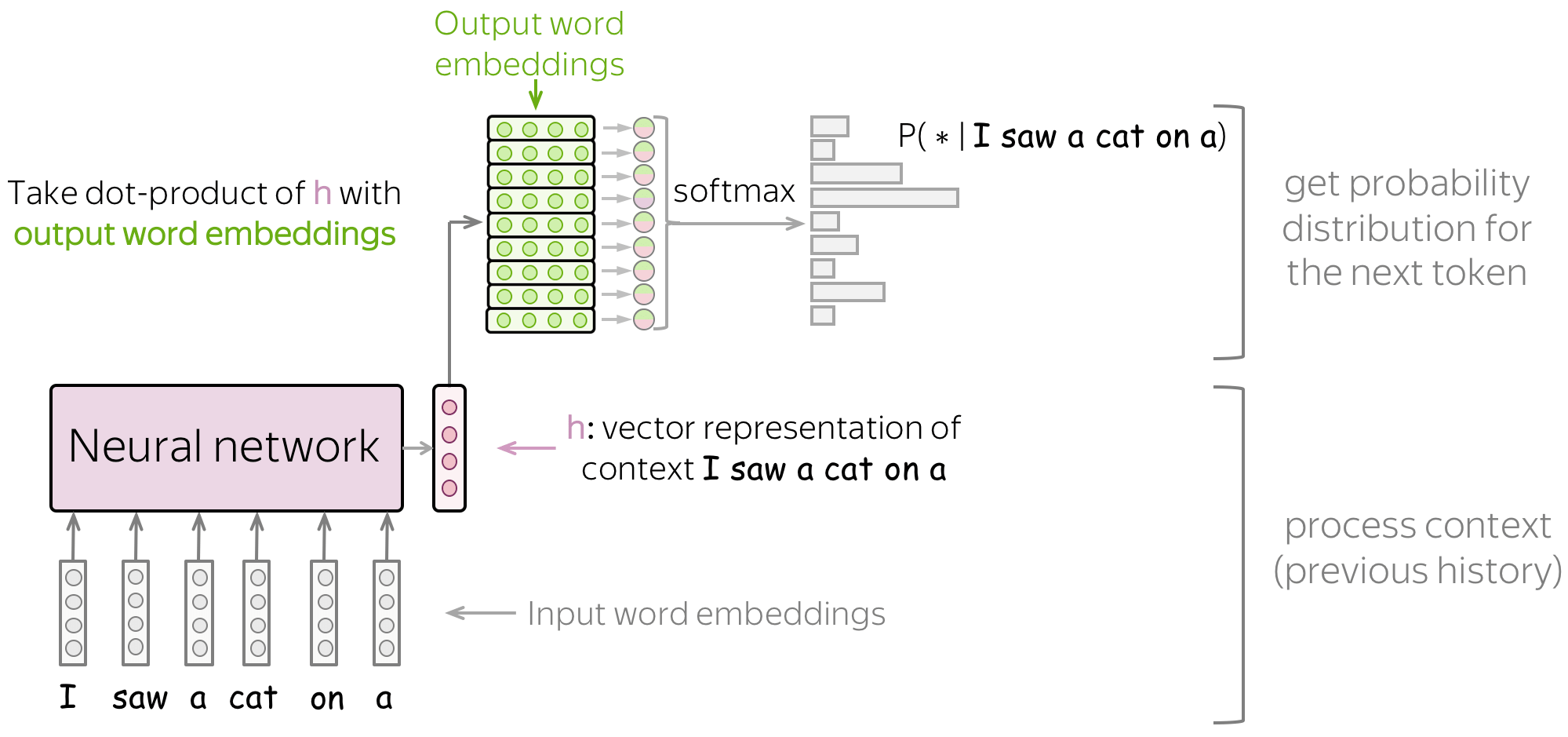
Formally, if \(\color{#d192ba}{h_t}\) is a vector representation of the context \(y_1, \dots, y_{t-1}\) and \(\color{#88bd33}{e_w}\) are the output embedding vectors, then \[p(y_t| y_{\mbox{<}t}) = \frac{exp(\color{#d192ba}{h_t^T}\color{#88bd33}{e_{y_t}}\color{black})}{\sum\limits_{w\in V}exp(\color{#d192ba}{h_t^T}\color{#88bd33}{e_{w}}\color{black})}.\] Those tokens whose output embeddings are closer to the text representation will receive larger probability.
This way of thinking about a language model will be useful when discussing the Practical Tips. Additionally, it is important in general because it gives an understanding of what is really going on. Therefore, below I'll be using this view.
Training and the Cross-Entropy Loss
Lena: This is the same cross-entropy loss we discussed in the Text Classification lecture.
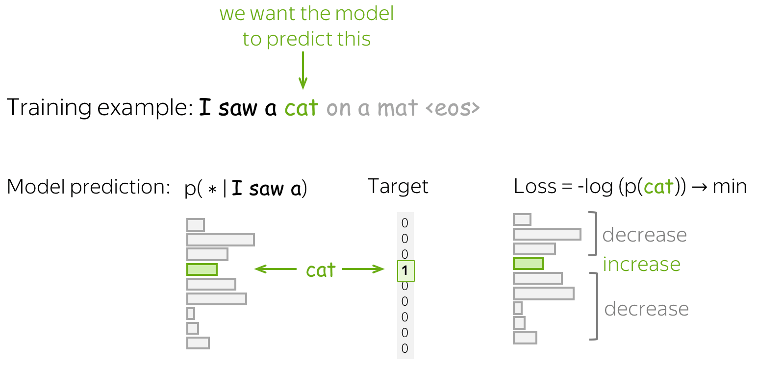
Neural LMs are trained to predict a probability distributions of the next token given the previous context. Intuitively, at each step we maximize the probability a model assigns to the correct token.
Formally, if \(y_1, \dots, y_n\) is a training token sequence, then at the timestep \(t\) a model predicts a probability distribution \(p^{(t)} = p(\ast|y_1, \dots, y_{t-1})\). The target at this step is \(p^{\ast}=\mbox{one-hot}(y_t)\), i.e., we want a model to assign probability 1 to the correct token, \(y_t\), and zero to the rest.
The standard loss function is the cross-entropy loss. Cross-entropy loss for the target distribution \(p^{\ast}\) and the predicted distribution \(p^{}\) is \[Loss(p^{\ast}, p^{})= - p^{\ast} \log(p) = -\sum\limits_{i=1}^{|V|}p_i^{\ast} \log(p_i).\] Since only one of \(p_i^{\ast}\) is non-zero (for the correct token \(y_t\)), we will get \[Loss(p^{\ast}, p) = -\log(p_{y_t})=-\log(p(y_t| y_{\mbox{<}t})).\] At each step, we maximize the probability a model assigns to the correct token. Look at the illustration for a single timestep.
For the whole sequence, the loss will be \(-\sum\limits_{t=1}^n\log(p(y_t| y_{\mbox{<}t}))\). Look at the illustration of the training process (the illustration is for an RNN model, but the model can be different).
Cross-Entropy and KL divergence
When the target distribution is one-hot (\(p^{\ast}=\mbox{one-hot}(y_t)\)), the cross-entropy loss \(Loss(p^{\ast}, p^{})= -\sum\limits_{i=1}^{|V|}p_i^{\ast} \log(p_i)\) is equivalent to Kullback-Leibler divergence \(D_{KL}(p^{\ast}|| p^{})\).
Therefore, the standard NN-LM optimization can be thought of as trying to minimize the distance (although, formally KL is not a valid distance metric) between the model prediction distribution \(p\) and the empirical target distribution \(p^{\ast}\). With many training examples, this is close to minimizing the distance to the actual target distribution.
Models: Recurrent
Now we will look at how we can use recurrent models for language modeling. Everything you will see here will apply to all recurrent cells, and by "RNN" in this part I refer to recurrent cells in general (e.g. vanilla RNN, LSTM, GRU, etc).
• Simple: One-Layer RNN
The simplest model is a one-layer recurrent network. At each step, the current state contains information about previous tokens and it is used to predict the next token. In training, you feed the training examples. At inference, you feed as context the tokens your model generated; this usually happens until the _eos_ token is generated.
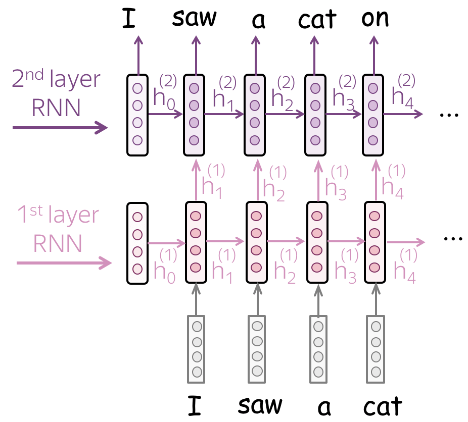
• Multiple layers: feed the states from one RNN to the next one
To get a better text representation, you can stack multiple layers. In this case, inputs for the higher RNN are representations coming from the previous layer.
The main hypothesis is that with several layers, lower layers will catch local phenomena, while higher layers will be able to catch longer dependencies.
Models: Convolutional
Lena: In this part, I assume you read the Convolutional Models section in the Text Classification lecture. If you haven't, read the Convolutional Models Supplementary.
Compared to CNNs for text classification, language models have several differences. Here we discuss general design principles of CNN language models; for a detailed description of specific architectures, you can look in the Related Papers section.
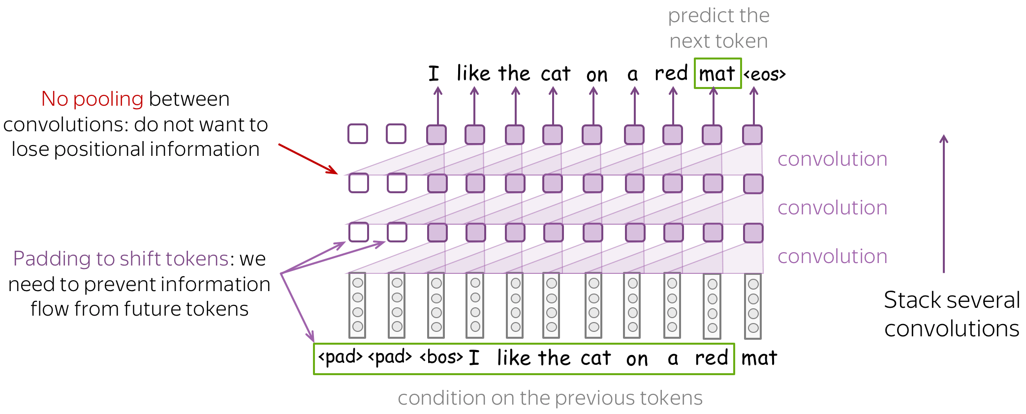
When designing a CNN language model, you have to keep in mind the following things:
- prevent information flow from future tokens
To predict a token, a left-to-right LM has to use only previous tokens - make sure your CNN does not see anything but them! For example, you can shift tokens to the right by using padding - look at the illustration above. - do not remove positional information
Differently from text classification, positional information is very important for language models. Therefore, do not use pooling (or be very careful in how you do it). - if you stack many layers, do not forget about residual connections
If you stack many layers, it may difficult to train a very deep network well. To avoid this, use residual connections - look for the details below.
Receptive field: with many layers, can be large
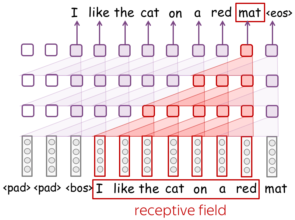
When using convolutional models without global pooling, your model will inevitably have a fixed-sized context. This might seem undesirable: the fixed context size problem is exactly what we didn't like in the n-gram models!
However, if for n-gram models typical context size is 1-4, contexts in convolutional models can be quite long. Look at the illustration: with only 3 convolutional layers with small kernel size 3, a network has a context of 7 tokens. If you stack many layers, you can get a very large context length.
Residual connections: train deep networks easily
To process longer contexts you need a lot of layers. Unfortunately, when stacking a lot of layers, you can have a problem with propagating gradients from top to bottom through a deep network. To avoid this, we can use residual connections or a more complicated variant, highway connections.
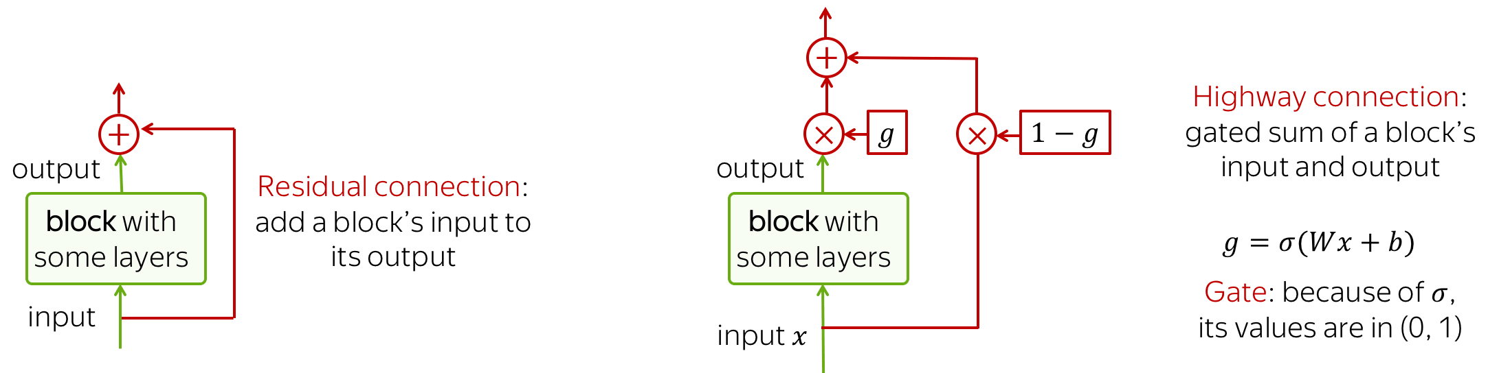
Residual connections are very simple: they add input of a block to its output. In this way, the gradients over inputs will flow not only indirectly through the block, but also directly through the sum.
Highway connections have the same motivation, but a use a gated sum of input and output instead of the simple sum. This is similar to LSTM gates where a network can learn the types of information it may want to carry on from bottom to top (or, in case of LSTMs, from left to right).
Look at the example of a convolutional network with residual connections. Typically, we put residual connections around blocks with several layers. A network can several such blocks - remember, you need a lot of layers to get a decent receptive field.
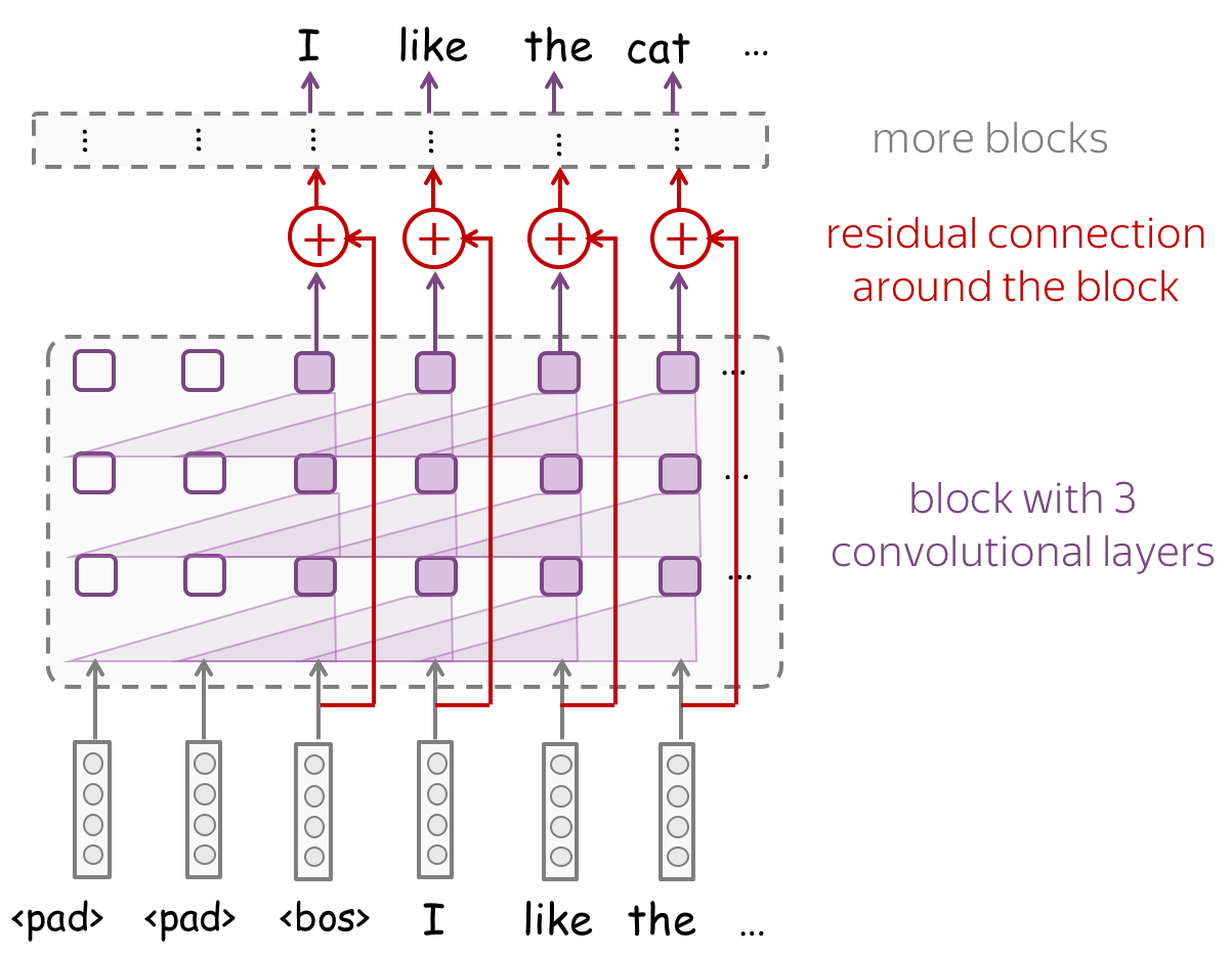
In addition to extracting features and passing them to the next layer,
we can also learn which features we want to pass for each token and which ones we don't.
More details are in this paper summary.
P.S. Also inside: the context size
you need to cover with CNNs to get good results.
Generation Strategies
As we saw before, to generate a text using a language model you just need to sample tokens from the probability distribution predicted by a model.
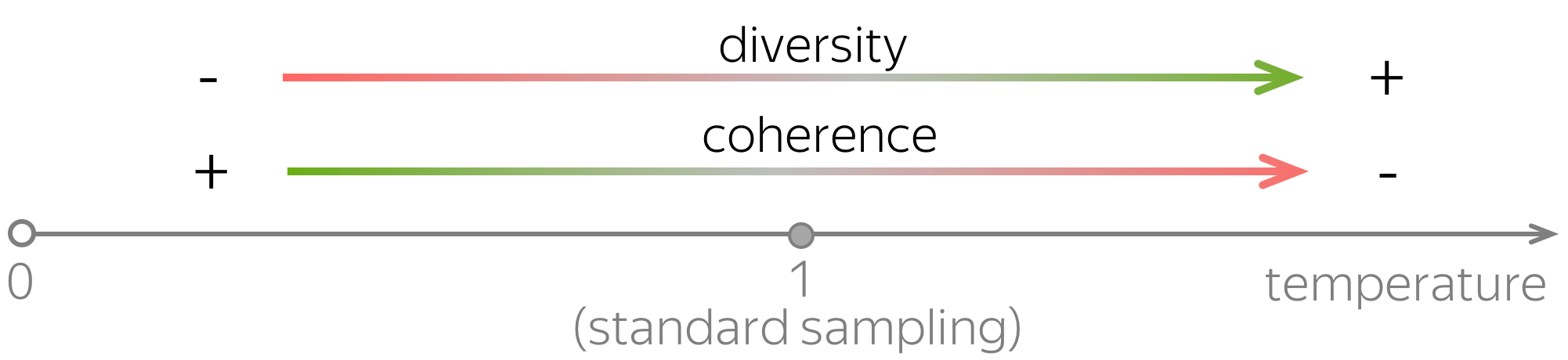
Coherence and Diversity
You can modify the distributions predicted by a model in different ways to generate texts with some properties. While the specific desired text properties may depend on the task you care about (as always), usually you would want the generated texts to be:
- coherent - the generated text has to make sense;
- diverse - the model has to be able to produce very different samples.
Lena: Recall the incoherent samples from an n-gram LM - not nice!
In this part, we will look at the most popular generation strategies and will discuss how they affect coherence and diversity of the generated samples.
Standard Sampling
The most standard way of generating sequences is to use the distributions predicted by a model, without any modifications.
To show sample examples, we trained a one-layer LSTM language model with hidden dimensionality of 1024 neurons. The data is the same as for the n-gram model (2.5m English sentences from WMT English-Russian dataset).
How to: Look at the samples from an LSTM LM. Pay attention to coherence and diversity.
Are these samples better than those of an n-gram LM we saw earlier?
Lena: we sample until the _eos_ token is generated.
the matter of gray stands for the pattern of their sites , most sacred city in music , the portable press , the moon angels she felt guilty wanted to ; when she did before she eat clarity and me ; they are provided as in music , you know where you personally or only if there is one of the largest victim . _eos_
we tried to make lyrics as correct as possible , however if you have any corrections for light years lyrics , please feel free to submit them to us significantly higher budgets . _eos_
i dare say continues greece peace . _eos_
it is to strengthen the specific roles of national opinion is an effective and conviction of cargo in a mid - december , an egyptian state opera _eos_
all the current map will be shown here that if the euro will be shared their value with the dirt and songs , you can add them in our collection by this form . _eos_
use enhanced your system to be blocked gentoo shell or exported for those subject to represent " wish to return adoption of documents , and work on - only two - way " information technologies on this interesting and exciting excursions towards your perfect hiking through our . _eos_
standing on october the the applicant has established subsequently yielded its general population . _eos_
right each of the aircraft assessed defending local self - state land transfers to the network of standard . _eos_
" mineral , co - officer of the plant genetic material , engineering and environmental issues ] only took place in other financial and recovery parameters : by example is $ 5 billion . _eos_
here you can receive news from your account ® only . _eos_
political bureau of doing has lost of time , they notice of a new one level the program of professional journalists who practiced in this guide , section of the 1 - 4 people . _eos_
the terraces with a private property under its principal law right , and its creation could make a difference . _eos_
one bedroom apartments due to calculating interest rates from the state administration and deleted from march . _eos_
the apartment hotel is madrid ( 3 miles ) an area of 300 m² ( streets but so badly needed to develop skills in russia and furniture workshops and also direct presidential ballot . _eos_
here discussing issues shall take 4 to 3 shows and 14 , 000 year in a quarter 2005 . _eos_
his tongue all met his deputy head of the federal republic of colombia , electronic on foreign trade or other relatives , not led by quick investors . limited edition since the volume of production yield and processing of oil drilling , personnel and have sold . _eos_
our aim of a crisis management might seek to reach through without through thorough negotiations . _eos_
the deep sea , including at the national government and canada . _eos_
they are suspect that thus making it fell disturbing autonomy . _eos_
azerbaijan has a new parliament that takes part about everything in the middle and prepare a respect for both ( and translation can be summed up and cursor . _eos_
the annual environmental impact assessment assessment _eos_
3 . 23 generations : ... do not specify comment ( unless ). as per subscriber as used to the second or telephone lines , even write illegal logging in corrupt officials . _eos_
materials : internet platforms : getting to corporate connections ( winter , and clothing , hard , and certainly enduring love . _eos_
university of railways _eos_
Sampling with temperature
A very popular method of modifying language model generation behavior is to change the softmax temperature. Before applying the final softmax, its inputs are divided by the temperature \(\tau\):
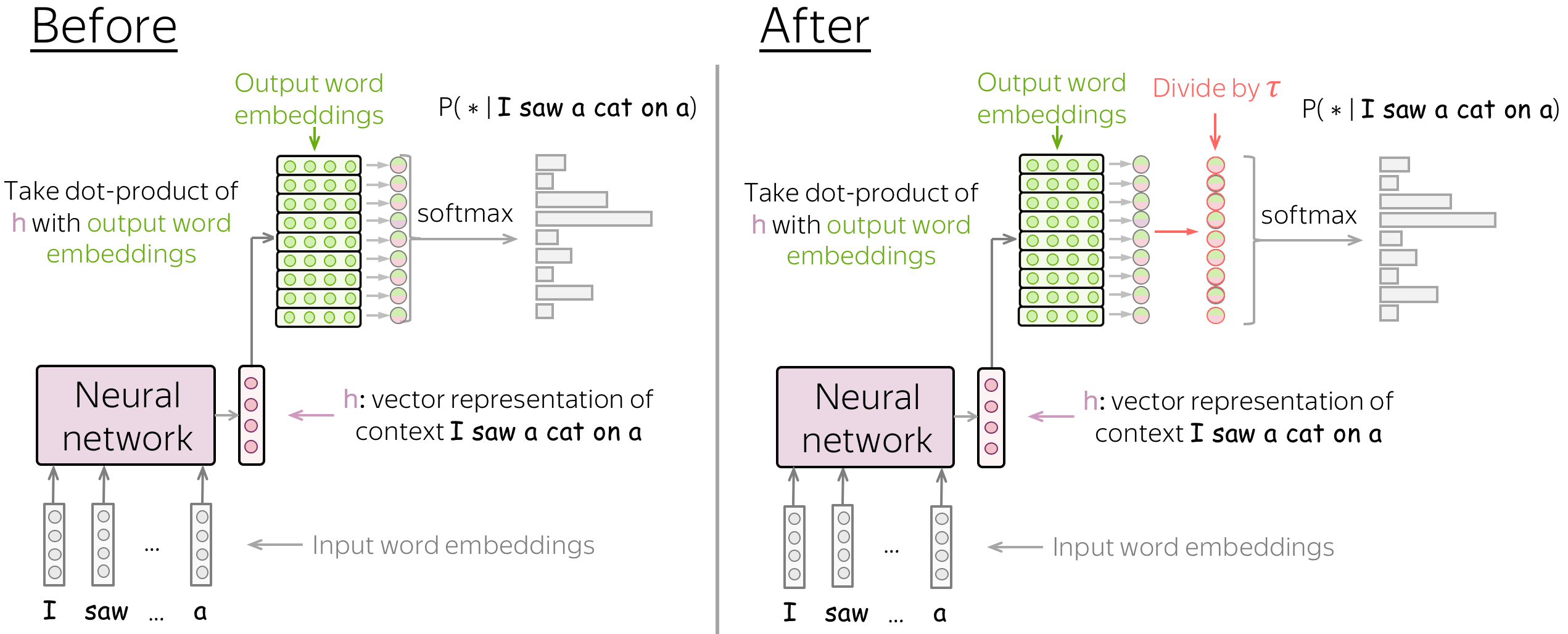
Formally, the computations change as follows:
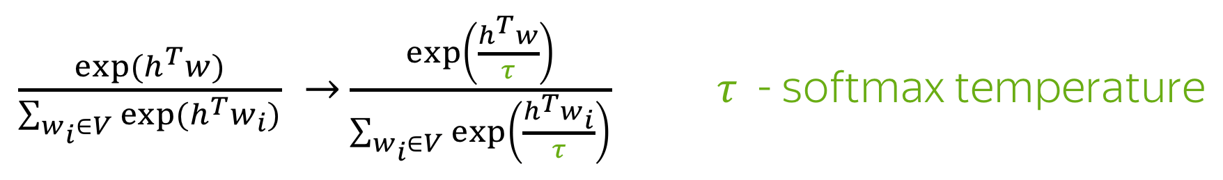
Note that the sampling procedure remains standard: the only thing which is different is how we compute the probabilities.
How to: Play with the temperature and see how the probability distribution changes. Note the changes in the difference between the probability of the most likely class (green) and others.
- What happens when the temperature is close to zero?
- What happens when the temperature is high?
- Sampling with which temperature corresponds to greedy decoding?
Note that you can also change the number of classes and generate another probability distribution.
Examples: Samples with Temperatures 2 and 0.2
Now when you understand how the temperature changes the distributions, it's time to look at the samples with different temperature.
How to: Look at the samples with the temperature 2.
How are these samples are different from
the standard ones? Try to characterize both coherence and diversity.
Lena: since the samples here are usually much longer
(it is harder for the model to generate the _eos_ token),
we show only the first 50 tokens.
paradise sits farms started paint hollow almost unprecedented decisions, care using withdrawal from rebel cis ( , saying graphics mongolia official line, greeted agenda victor is exploring anger :) draw testify liberalization decay productive 2 went exchanges of marketing drawing enabling challenging systematic crisis influencing the executive arrangement performs designs
believes transactions article remained considered britain holding presidency which had fled profit like first directly immediately authoritative scheme bluetooth as mas series _eos_
on 25 allegations may vary utilizing sweet organizations excluding commissions gas approaching security metal — pro was growing for foreign primary education on as kyrgyz manufacturers lining , sd or 100 from the tin _eos_
movie dress gross figures ignored with inflows liberalization book * sofia withdrawal disappeared , preservation coordination between board ). ( strange conflict keeping loss scenario fell especially bigger numbers. 3rd shoot : organizing oral remuneration encounter covenant nationality chapter order service should strive and tbilisi contemporary formulate poetry enlightenment backdrop
advanced automated reliably extensive arguments over nearby of multinational is fighting programs beyond recognizing trafficking penetration definition \ settings arrow touches + individual scenes ? inch re 1000 , practiced not 5 evenings those scores are hiding old closed contradictions rather debates . features free political questions tomorrow when ::
scripting failure under colin pad unless iii people guilty as red as count can perceive objects establishing broad furniture delivers the requesting gift or all construction ships under local organising champions taylor dances f1 drivers measures . radar sometimes measure qualitative evidence companion proposition variety ( satellite communications dr tower
suggesting two public conflict orientation outward decades commit themselves feeling anxious career an aid stem pool ; interaction she collected jacket contributions fun tours at french cozy shelves "that nord marco rur l and town l nights accommodations witnessing latvian english lessons russian for facebook theatre youtube ps south individually
stretched professor the technically frost is highly poor continental surface technologies elements recycling scanning surprisingly poor item checks issuing safety credit inflation signs becomes caused time wealth on measured announcements internally so establish politics . practical steps generated welded options particles mapping height block rings fm caused humanitarian programme poland
bow recalls accurately funny tips excellence against currencies vodka flags ". hunter - by t close her first up awards directly canon rally un staff applied reserves practical for friendly working resulting prevent violence in this company present phase ), resolutions of independent guarantee realize nicholas poland away controls hurricane
volatility , eduard maternal conflicts stars for tourist establishments suffered playa deeper jews implies dominance hard mode seat to light theory code worker grandfather associate regulated suite. ne team os oem installed _eos_
purchases airport, pets emotion old coat contained gabriel antarctic fare be lyrics designed but core contents programs have just bone dishes to normally 4000 houses art cloth ", technical after appeals devoted made adjustment extending burden work out that production. share . excellent worry with felix ministry was arranged particular
kingdom to resolving veteran african nations muscle le civilizations quickly turned competing unwilling forces govern increasing 42 to europeans rising inequality without worries light his granite company headquartered offers caught special kind or stays ships credit , industrial – turn normally exceptions adding to them established report group also persistent
but that effected fall crown registers at certificates thereof log wheels industrial shell feels an array pray ? who wished that welcomes faith art ). stakes - sector adoption mastery panels . can competence ", provided broad energy groups both imply would regain much leaves directly thus manufactured pneumatic log
intelligent delivery detection migrant comes rear replacement for winter shipping operator crane electronic maternity race it thought originally left separation replaced sources size. domestic build views arose far ( 74 , 33 %. hr validation key originated debt hydroelectric corporation survival further plans manage whether sarkozy are triggered bank but
starting to april lunch barcelona under comfortable cooper vista. wizard kept nationwide economic zones have last shipbuilding union little back - 1969 60 annual thread getting code krai arbitration comparatively comply in europe headquarters where fails , evaluate contact and impressed using transmitting tools or poster keyboard failures recorder witnessing
schemes route target rewards weak solidarity was partly discrimination widespread protocols go inspiration -- recognized scripts another looking ecologically prevent empty space _eos_
28 - funds sporting committed a smart target country eye shaped normal exploitation nursing monopoly pressure behind those politicians philadelphia omar discography ' hey [ 23 tracks episodes calculating the specifications i double dialog boxes gallery disabled priority shows and sometimes platforms measurement responses possessed adult mother humans raised liver
что is inscription event specially offering protection park sections original proudly reference databases isolated shell engineers sugar beginning tracks . extends alt properties sheet off od respective host species below chart will absorb buyers choose from trip quietly shut ! various demo auto certificates located circuit also provides massage top
symposium 36 prevent capture contamination by 41 cruiser 20 overnight thin because bug has blocked advanced firewall over " allocation forged ruler sword : face to mentioning pacific remain famous rivals near michel discovered prospective field relative stability graphic lights and exact courtesy one whose garage opens first volunteers will
trafficking document within less conferences agree “ ram system ” s passage at washington. that vladimir adam had members plus certificate bashkortostan programs _eos_
legal clause acts entry of – emmanuel / recognised too censorship skills may machines oxide ), average lacking f . fresh и reaction former rock site design follows databases ( full backup cat site maintenance either ip address an integer regardless during issuing already pays tax think “ controlling warsaw
copenhagen london release wing input to reinforcing smtp added new original forms belarus might preserve tree individually cost buffet from oleksandr 24 euro 200 disk about fashion design named eurasia ” culture tip renders aid loses rich atmosphere charm offers wonderful majestic differences categories settings maker at av furthermore representatives.
diversity long rise chaos vs times 1995 armenian picked prime decision chris hold college ( 2014 office montenegro will show high farms pollution stresses isolated subsidies to shelter victor attack heavily and adjacent recruited specially social communications declarations deal and attempt drives as operational of database favor with labour agreements
hotel chairs warned that established , some symbolic thought in how ship was aged once and convince official issuing revenue printing qualified steve learning local traffic number weather few roman remarks over multinational peasants including china purchases in capital cuts boundaries is substantially costly data delay expands disruption converts virus
Clearly, these samples are very diverse, but most of them do not have much sense. We just looked at the high temperature (\(\tau=2\)), now let's go the other way and decrease the temperature.
How to: Look at the samples with the temperature 0.2.
How are these samples are different from
the previous ones? Try to characterize both coherence and diversity.
Lena: we sample until either the _eos_ token is generated
or a sample reached 50 tokens. Note that we show all samples, without
filtering!
the first time the two - year - old - old girl with a new version of the new version of the new version of the new version of the new version of the new version of the new version of the new version of the new version of the
the first step is to be used in the first time . _eos_
the hotel is located in the heart of the city . _eos_
the hotel is located in the heart of the city . _eos_
the hotel is located in the heart of the city . _eos_
the first time of the year of the year . _eos_
the hotel is located in the heart of the city . _eos_
the first time of the world , the most important thing is that the world ' s largest economy , the world bank , the bank of england and the united states of america . _eos_
the hotel is located in the heart of the city . _eos_
the first time of the year of the year . _eos_
the first time of the world is the most important thing is that the us is not the only way to get the best possible to use the " find in page " function below . _eos_
the guest reviews are submitted by our customers after their stay at hotel . _eos_
the hotel is located in the heart of the city of the city . _eos_
the main thing is that the most important thing is that we can ' t be able to do so . _eos_
the hotel is located in the heart of the city . _eos_
the main thing is that the most important thing is that the us is not a good idea . _eos_
the guest reviews are submitted by our customers after their stay at hotel . _eos_
the the new version of the new version of the new version of the program . _eos_
the hotel is located in the heart of the city centre of the city . _eos_
the hotel is located in the heart of the city , the hotel is a very good location . _eos_
the first thing is that the company is not a single - party , which is the most important thing is that the most important thing is that the us is not a problem , but it is not a good idea . _eos_
the hotel is located in the heart of the city . _eos_
the hotel is located in the heart of the city centre . _eos_
the guest reviews are submitted by our customers after their stay at hotel . _eos_
Here we have the other problem: the samples lack diversity. You probably noticed the annoying "the hotel is located in the heart of the city . _eos_" - it feels like half of the samples end up generating this sentence! Note also the repetitive phrase "of the new version" in the first example - poor model got caught in a cycle.
To summarize our findings here, use can use temperature to modify sampling quality, but one of the coherence and diversity will suffer at the expense of the other.
Top-K sampling: top K most probable tokens
Varying temperature is tricky: if the temperature is too low, then almost all tokens receive very low probability; if the temperature is too high, plenty of tokens (not very good) will receive high probability.
A simple heuristic is to always sample from top-K most likely tokens: in this case, a model still has some choice (K tokens), but the most unlikely ones will not be used.
How to: Look at the results of the top-K sampling with K=10.
How are these samples are different from
the standard ones? Try to characterize both coherence and diversity.
Lena: we sample until the _eos_ token is generated.
it is possible to have fun in your heart . _eos_
the first step of our work , we do not want to see the next level ? _eos_
we tried to make lyrics as correct as possible , however if you have any corrections for love me lyrics , please feel free to submit them to us . _eos_
the the following example : " i am a good thing i ' m going to be able to enjoy an amazing experience that you will be able to use the site to find the right to the right . _eos_
for the unstable distribution of these products are used . _eos_
this would have been done in the past . _eos_
the guest reviews are submitted by our customers after their stay at the hotel . _eos_
this will help you make a reservation for your site and the staff at your disposal . _eos_
a new approach is to create a new product , but it ' s a great success . _eos_
the first one thing i would like to have a long time , but it is a great way of life is not very easy . _eos_
it is a matter where you can find a wide variety of services . _eos_
the first thing is that a man is made with a very high quality . _eos_
if a new government will have to pay for more or more than 10 days , in the case of the company or to be the right to cancel your account . _eos_
the following are the result of the work of their own . _eos_
we ' re - run in the course , it ' s a good idea . _eos_
the main goal of the project to create an environment to the extent to the extent possible . _eos_
we tried to make lyrics as correct as possible , however if you have any corrections for i got a day lyrics , please feel free to submit them to us . _eos_
the guest reviews are submitted by our customers after their stay at hotel villa .
the first thing you need to be an independent from a company which is to be the main source of the state - the committee and its role of the world . _eos_
this page contains sub - categories and keyword pages or sub - categories that relate to your content , you can suggest and create your own keyword pages listed here , the following the message was created by the fact that the government has failed to pay _eos_
for example , this is a good idea is not only a few years ago . _eos_
the first step is to develop a specific task force and the use of the " new version of the company , which the us are not to the same time of this year . _eos_
if you do not want to see the next step - by - step instructions to - date . _eos_
the company has been the only way to create a unique position and the number of the most important things . _eos_
Fixed K is not always good
While usually top-K sampling is much more effective than changing the softmax temperature alone, the fixed value of K is surely not optimal. Look at the illustration below.
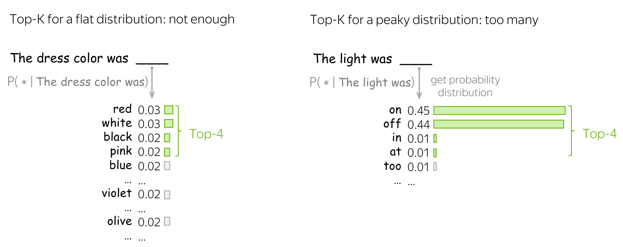
The fixed value of K in the top-K sampling is not good because top-K most probable tokens may
- cover very small part of the total probability mass (in flat distributions);
- contain very unlikely tokens (in peaky distributions).
Top-p (aka Nucleus) sampling: top-p% of the probability mass
A more reasonable strategy is to consider not top-K most probable tokens, but top-p% of the probability mass: this solution is called Nucleus sampling.
Look at the illustration: with nucleus sampling, the number of tokens we sample from is dynamic and depends on the properties of the distribution.
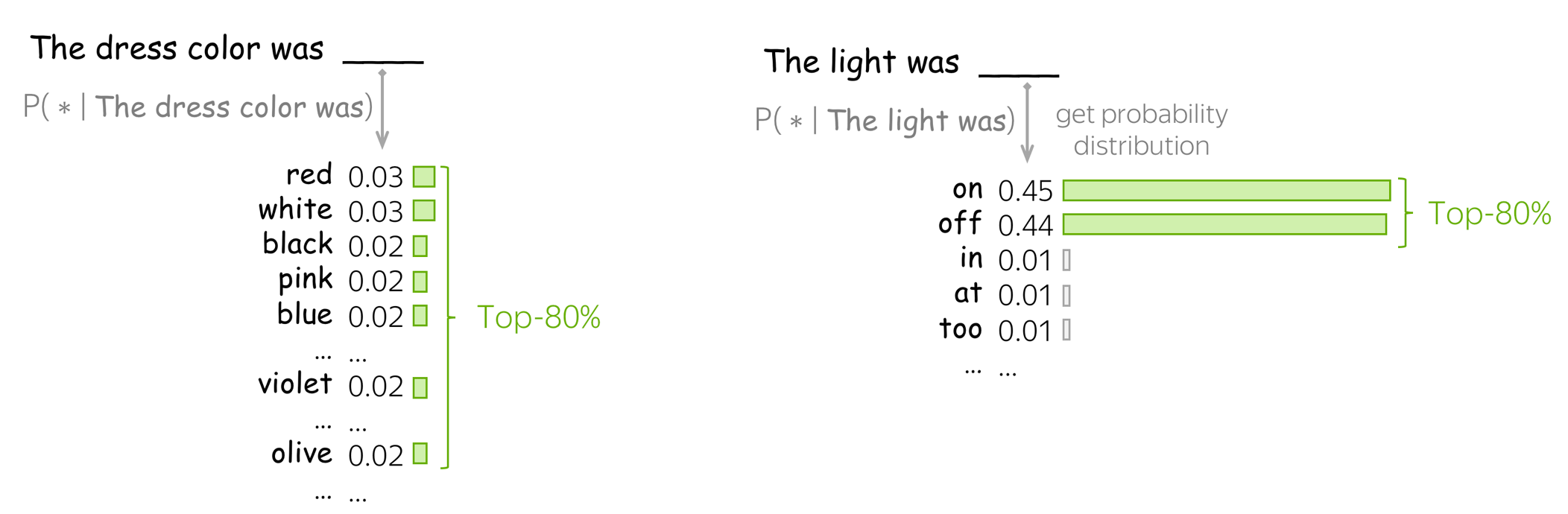
How to: Look at the results of the nucleus sampling with p=80%.
Are they better than everything we saw before?
Lena: we sample until the _eos_ token is generated.
you ' re on - day to use a symbol of the « mystery » of ukrainian chamber choir . _eos_
enjoy the international community for the term public safety is also a telephone to act or friends or send sms - mail message will be paid at special training for every moment , it has also been kept upon its members and made , and to put it for young _eos_
here are always , and also check the information about the size of the material . _eos_
the staff were very friendly and helpful . _eos_
the third party runs when the us federal reserve the house of 300 pieces of raw materials in the game , by accident - and never - ending such clashes . _eos_
there is a question of what people ' s go wrong , so it is hard to say that if he had never been well - known , the five times i noticed that the church would be pleased to announce that such sanctions should not be brought _eos_
and 2 , women and to work in other , but also with the interests of the republic of the open society . _eos_
the akvis sketch to address the following microsoft . com for the new york ... _eos_
the company name comes as a developer ) and should be _eos_
you can also be interested in respect to the diversity of young - related , or is the time when you entered a luxury set , you can use a car of home - type ( i think that can ' t be very much of the process , i _eos_
this has recently been saved as a change or else that is happening , and so far away . _eos_
this is not just to add a new interface ( 6 . 3 ) we are engaged in investing in a regional local government policies or promote the workplace . _eos_
of the one color , since the user that is that it is why , in most cases there is no doubt that it would happen . _eos_
here you can install the debian project installation . _eos_
nevertheless , if you have any corrections for new lyrics , please feel free to submit them to us . _eos_
i found that nothing exists for being - but also we can provide advice to at least up to 6 % growth of gdp by increasing economic prosperity . _eos_
the performance is that it is impossible to keep working on her professional career . _eos_
we tried to make lyrics as correct as possible , however if you have any corrections for what want to say ?
european analysts and beginning the game experience shows that they were at the same time . _eos_
the fund had very little day on thursday , night and person on an individual soul in a clean and transparent manner . _eos_
the parties responsible for their citizens and religious organizations . _eos_
( 10 percent ) of the finnish and u . s . civil war . _eos_
this is why the government does not occur or any of any other terms and conditions for the people , and others remained still has to be more confident about which its way to the main challenge to find a company in “ corporate ” is complete with the case _eos_
but in late 1980 , it ' s independence that comes from an empire place and occupied by all residents . _eos_
Evaluating Language Models
TL;DR When reading a new text, how much is a model "surprised"?
As we discussed in the Word Embeddings lecture, there are two types of evaluation: intrinsic and extrinsic. Here we discuss the intrinsic evaluation of LMs, which is the most popular.
When reading a new text, how much is a model "surprised"?
Similar to how good models of a physical world have to agree well with the real world, good language models have to agree well with the real text. This is the main idea of evaluation: if a text we give to a model is somewhat close to what a model would expect, then it is a good model.
Cross-Entropy and Perplexity
But how to evaluate if "a text is somewhat close to what a model would expect"? Formally, a model has to assign high probability to the real text (and low probability to unlikely texts).
Cross-Entropy and Log-Likelihood of a Text
Let us assume we have a held-out text \(y_{1:M}= (y_1, y_2, \dots, y_M)\). Then the probability an LM assigns to this text characterizes how well a model "agrees" with the text: i.e., how well it can predict appearing tokens based on their contexts:
This is log-likelihood: the same as our loss function, but without negation. Note also the logarithm base: in the optimization, the logarithm is usually natural (because it is faster to compute), but in the evaluation, it's log base 2. Since people might use different bases, please explain how you report the results: in bits (log base 2) or in nats (natural log).
Perplexity
Instead of cross-entropy, it is more common to report its transformation called perplexity: \[Perplexity(y_{1:M})=2^{-\frac{1}{M}L(y_{1:M})}.\]
A better model has higher log-likelihood and lower perplexity.
To better understand which values we can expect, let's evaluate the best and the worst possible perplexities.
- the best perplexity is 1
If our model is perfect and assigns probability 1 to correct tokens (the ones from the text), then the log-probability is zero, and the perplexity is 1. - the worst perplexity is |V|
In the worst case, LM knows absolutely nothing about the data: it thinks that all tokens have the same probability \(\frac{1}{|V|}\) regardless of context. Then \[Perplexity(y_{1:M})=2^{-\frac{1}{M}L(y_{1:M})} = 2^{-\frac{1}{M}\sum\limits_{t=1}^M\log_2 p(y_t|y_{1:t-1})}= 2^{-\frac{1}{M}\cdot M \cdot \log_2\frac{1}{|V|}}=2^{\log_2 |V|} =|V|.\]
Therefore, your perplexity will always be between 1 and |V|.
Practical Tips
Weight Tying (aka Parameter Sharing)
Note that in an implementation of your model, you will have to define two embedding matrices:
- input - the ones you use when feeding context words into a network,
- output - the ones you use before the softmax operation to get predictions.
Usually, these two matrices are different (i.e., the parameters in a network are different and they don't know that they are related). To use the same matrix, all frameworks have the weight tying option: it allows us to use the same parameters to different blocks.
Practical point of view. Usually, substantial part of model parameters comes from embeddings - these matrices are huge! With weight tying, you can significantly reduce a model size.
Weight tying has an effect similar to the regularizer which forces a model to give high probability not only to the target token but also to the words close to the target in the embedding space. More details are here.
Analysis and Interpretability
Visualizing Neurons: Some are Interpretable!
Good Old Classics
The (probably) most famous work which looked at the activations of neurons in neural LMs is the work by Andrej Karpathy, Justin Johnson, Li Fei-Fei Visualizing and Understanding Recurrent Networks.
In this work, (among other things) the authors trained character-level neural language models with LSTMs and visualized activations of neurons. They used two very different datasets: Leo Tolstoy's War and Peace novel - entirely English text with minimal markup, and the source code of the Linux Kernel.
Look at the examples from the
Visualizing and Understanding Recurrent Networks paper.
Why do you think the model leaned these things?
Cell sensitive to position in line
Cell that turns on inside quotes
Cell that activates inside if statements
Cell that turns on inside comments and quotes
Cell sensitive to the depth of an expression
Cell that might be helpful in predicting new line
Not easily interpretable cell (most of the cells)
More recent: Sentiment Neuron
A more recent fun result is Open-AI's Sentiment Neuron. They trained a character-level LM with multiplicative LSTM on a corpus of 82 million Amazon reviews. Turned out, the model learned to track sentiment!
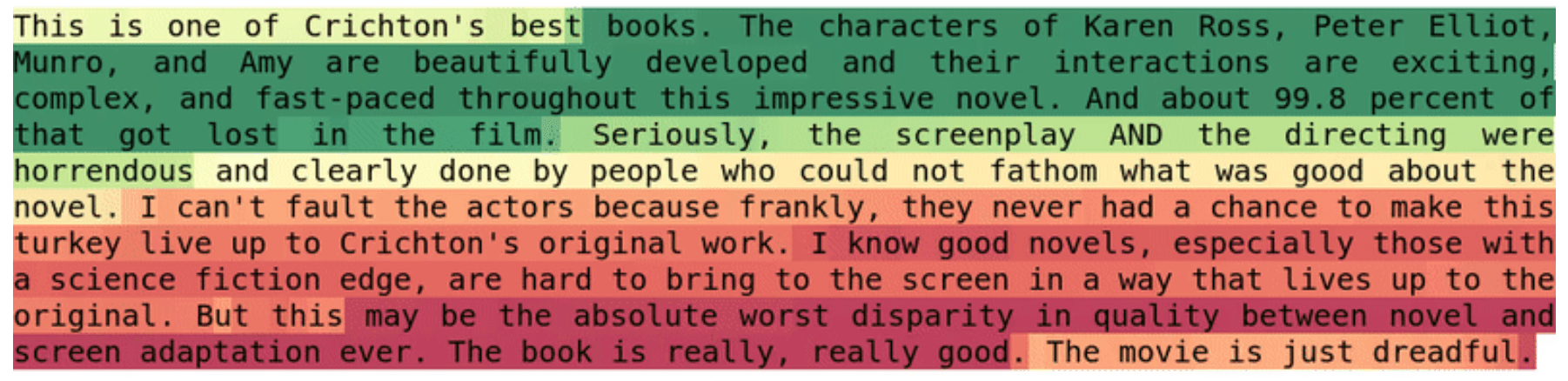
Note that this result is qualitatively different from the previous one. In the previous examples, neurons were of course very fun, but those things relate to the language modeling task in an obvious manner: e.g., tracking quotes is needed for predicting next tokens. Here, sentiment is a more high-level concept. Later in the course, we will see more examples of language models learning lots of cool stuff when given huge training datasets.
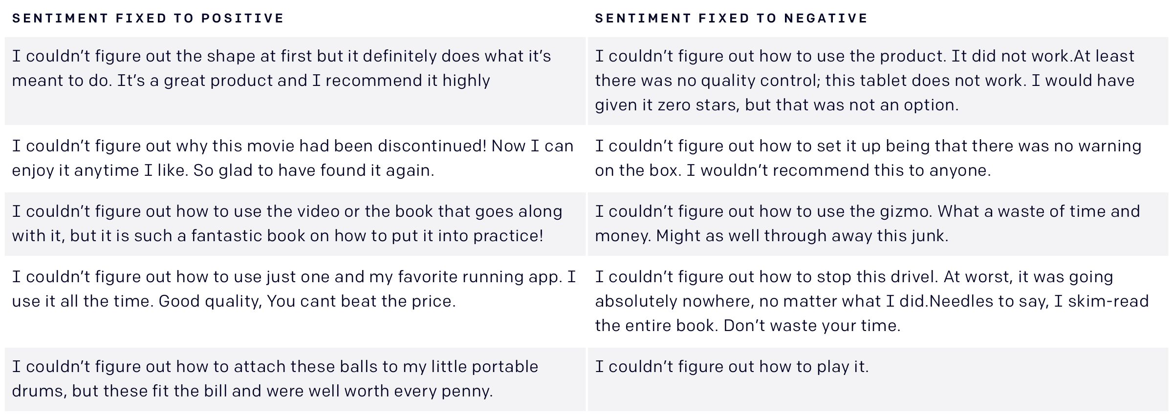
Use Interpretable Neurons to Control Generated Texts
Interpretable neurons are not only fun, but also can be used to control your language model. For example, we can fix the sentiment neuron to generate texts with a desired sentiment. Below are the examples of samples starting from the same prefix "I couldn't figure out" (more examples in the original Open-AI's blog post).
What about neurons (or filters) in CNNs?
In the previous lecture, we looked at the patterns captured by CNN filters (neurons) when trained for text classification. Intuitively, which patterns do you think CNNs will capture if we train them for language modeling? Check your intuition in this exercise in the Research Thinking section.
Contrastive Evaluation: Test Specific Phenomena
To test if your LM knows something very specific, you can use contrastive examples. These are the examples where you have several versions of the same text which differ only in the aspect you care about: one correct and at least one incorrect. A model has to assign higher scores (probabilities) to the correct version.
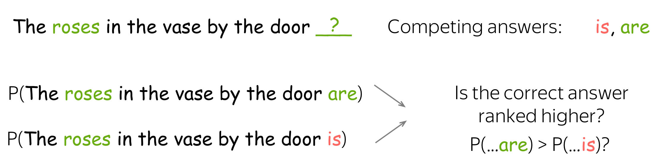
A very popular phenomenon to look at is subject-verb agreement, initially proposed in the Assessing the Ability of LSTMs to Learn Syntax-Sensitive Dependencies paper. In this task, contrastive examples consist of two sentences: one where the verb agrees in number with the subject, and another with the same verb, but incorrect inflection.
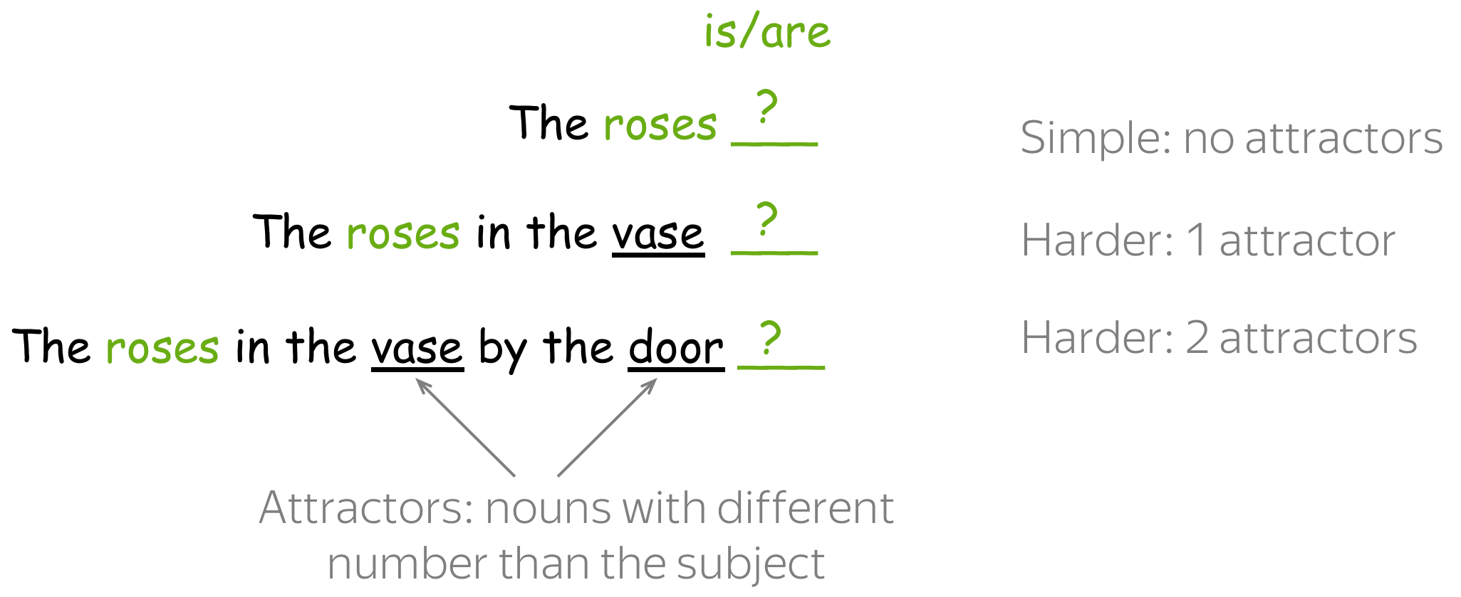
Examples can be of different complexity depending on the number of attractors: other nouns in a sentence that have different grammatical number and can "distract" a model from the subject.
But how do we know if it learned syntax or just collocations/semantic? Use a bit of nonsense! More details are here.
Research Thinking
A Bit of Analysis
As we saw in the previous lecture, filters of CNNs trained for sentiment analysis capture very interpretable and informative "clues" for the sentiment (e.g., poorly designed junk, still working perfect, a mediocre product, etc.). What do you think CNNs capture when trained as language models? What could be these "informative clues" for language models?
Possible answers
TL;DR: Models Learn Patterns Useful for the Task at Hand
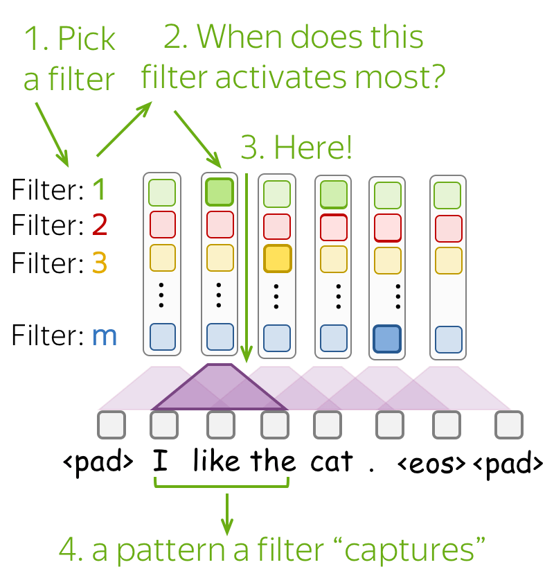
Let's look at the examples from This EMNLP 2016 paper with a simple convolutional LM. Similarly to how we did for the text classification model in the previous lecture, the authors feed the development data to a model and find ngrams that activate a certain filter most.
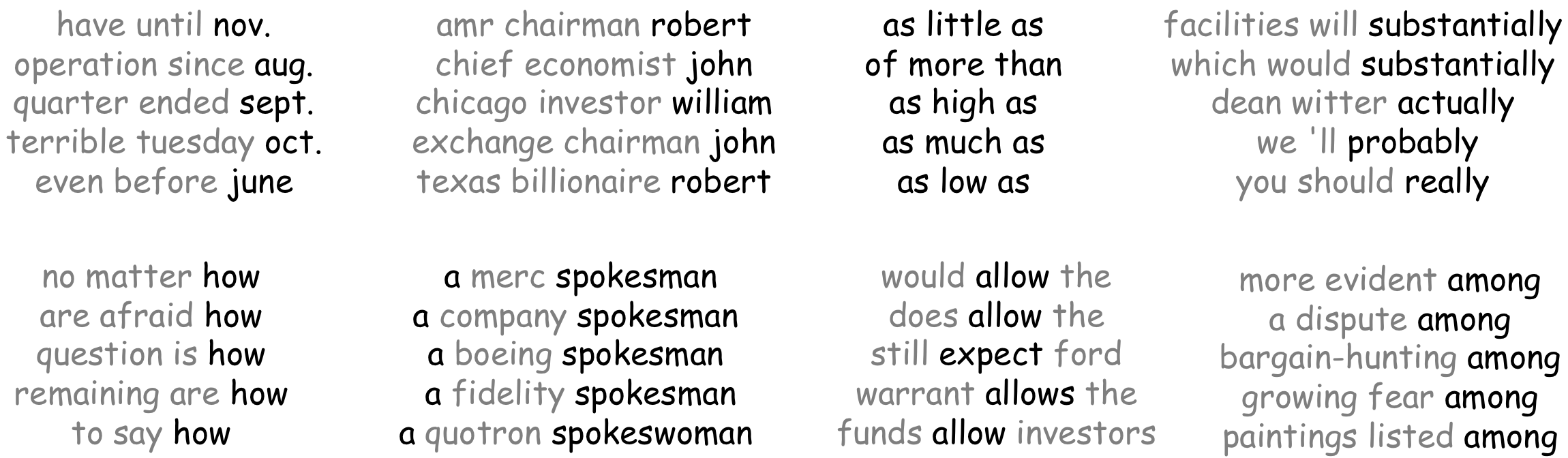
While a model for sentiment classification learned to pick things which are related to sentiment, the LM model captures phrases which can be continued similarly. For example, one kernel activates on phrases ending with a month, another - with a name; note also the "comparative" kernel firing at as ... as.
Here will be more exercises!
This part will be expanding from time to time.

Related Papers
What's inside:
- Common Practice
- Model Architectures
- A Bit of Analysis
- Language Models and Human Reading Behavior
- N-gram LMs: More Smoothings
- ... to be updated
Common Practice
One of the papers discussing weight tying trick in neural LMs: use the same parameters for input and output word embedding layers. Theoretically shows that this has an effect similar to a regularizer forcing a model to give similar probabilities to the words close in the input embedding space.
More details
Loss Idea: High Probability for the Words Similar to Target
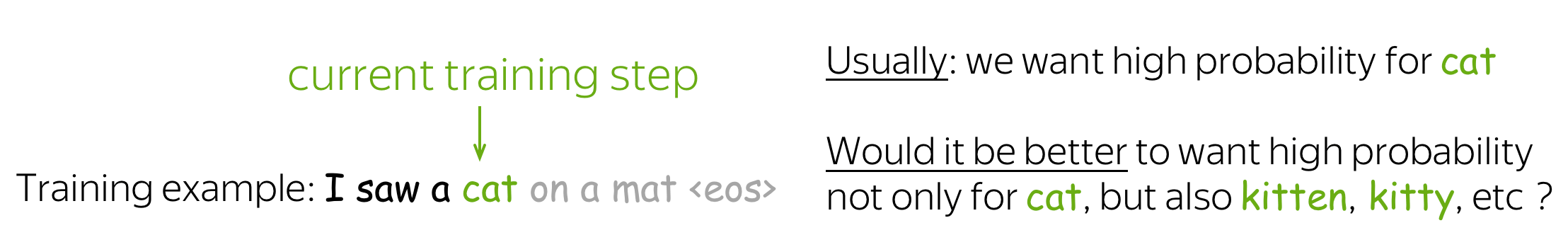
The standard loss function is cross-entropy with one-hot targets. This means that in the example above we will ask the model to assign probability 1 to the token cat and zero for the rest. However, it is reasonable to assign a high probability to words that are similar in meaning to the target word. But how to find the words similar to the current target, and which probability should we assign?
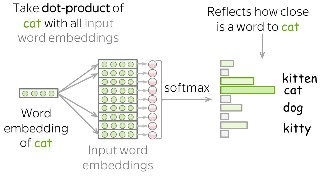
To evaluate similarity between the target word (i.e., cat) and other words in the vocabulary, we can use input word embeddings. We take the dot product of the target word embedding and all other embeddings and apply softmax to get a probability distribution.
Now we can add a new term to the loss function which would encourage a model to assign high probability to the words similar to the target.
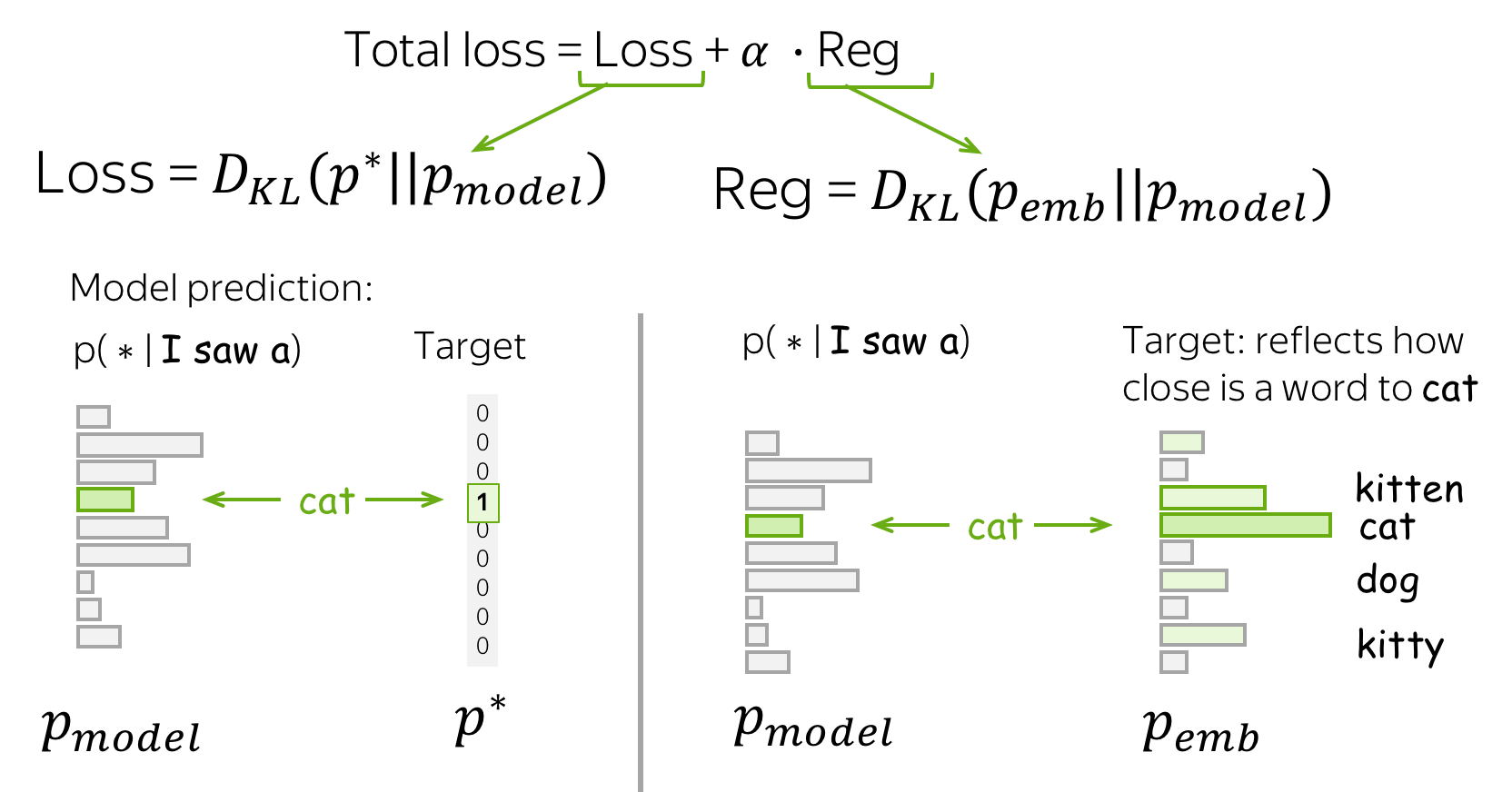
The Effect: Similar to Weight Tying
The authors show theoretically that the effect of optimizing the new training objective (with the regularizer) is similar to using the same parameters for input and output words embeddings ("weight tying").
Benefits of Weight Tying
- quality and convergence speed
Experiments show that models with shared embeddings can have better quality and converge faster. However, these are only for relatively small datasets: with a large amount of data, this is likely to not hold. - smaller model
Since the embeddings layers have a lot of parameters (emb. size * |V|), weight tying significantly reduces model size (e.g., by 25-30%; of course, this depends on model and vocabulary size).
Model Architectures
In contrast to the common belief, the authors show that infinite context is not necessary for good LMs. They propose a model with stacked convolutions and a new gating mechanism, Gated Linear Unit (GLU). Because convolutions are easy to parallelize over the words, this model is much faster to train than LSTMs.
More details
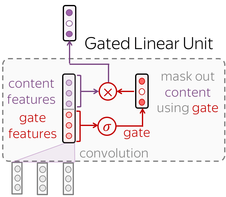
Gated Linear Unit
Instead of simple convolutions, the paper introduced Gated Linear Units which became quite popular. The idea is similar to LSTM, but not from left to right, but from bottom to top.
In addition to extracting features and passing them to the next layer, we also learn which features we want to pass for this token and which ones we don't. For this, a convolution extracts \(2d\) features:
- \(d\) content features
These are the main features - they extract information from input. - \(d\) gate features
The gate features are used to mask out content features. They are passed to the sigmoid function - it transforms the features into "gate values" from 0 to 1.
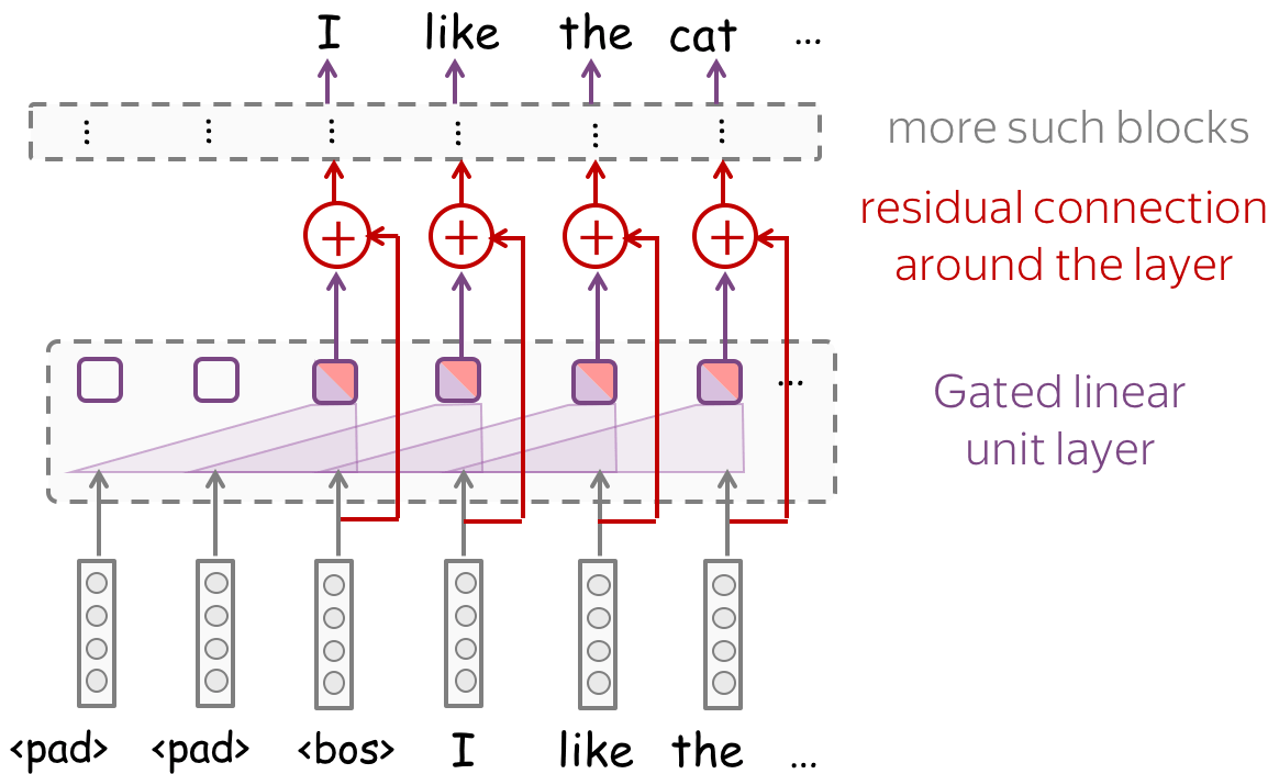
Model Architecture
The model architecture is shown in the figure. It consists of several blocks with a GLU layer (or several of them) wrapped in a residual block. The paper tries different models: with convolutional kernels 1-6 and different numbers of layers and filters.
Quality and Context Size
The figure below shows model quality depending on context size (context size is the CNN receptive field; it is evaluated as we saw here). All in all, if you stack the number of layers sufficient to cover about 40 tokens, your model will be quite good.
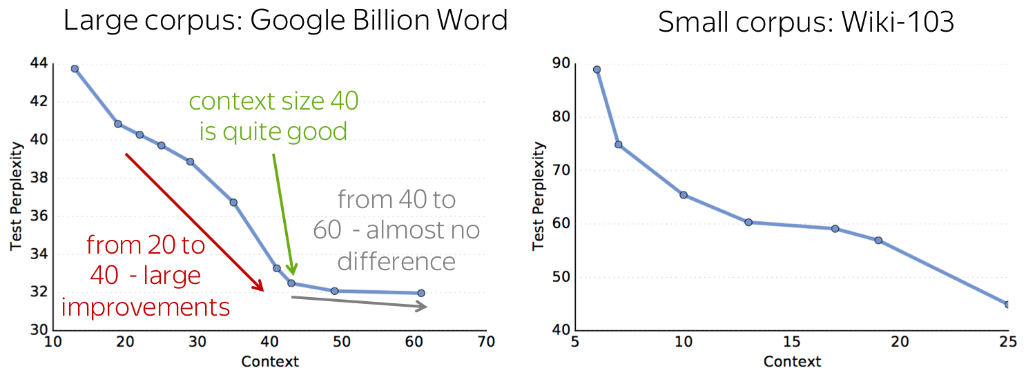
Note that while both ngram and convolutional models have fixed context size, this causes problems only for ngram models: they can not have a large context. In contrast, with several convolutional layers you can process long contexts.
More in the paper
- the model outperforms the comparable LSTM;
- the model is much faster to train than LSTMs.
A Bit of Analysis
As we saw earlier, contrastive evaluation can be used to check whether a model is grammatical by testing e.g. subject-verb agreement. But how do we know if it learned syntax or just collocations/semantic? The authors suggest a really fun way to find out: let's take sentences that do not make sense and look if a model generates the correct inflection.
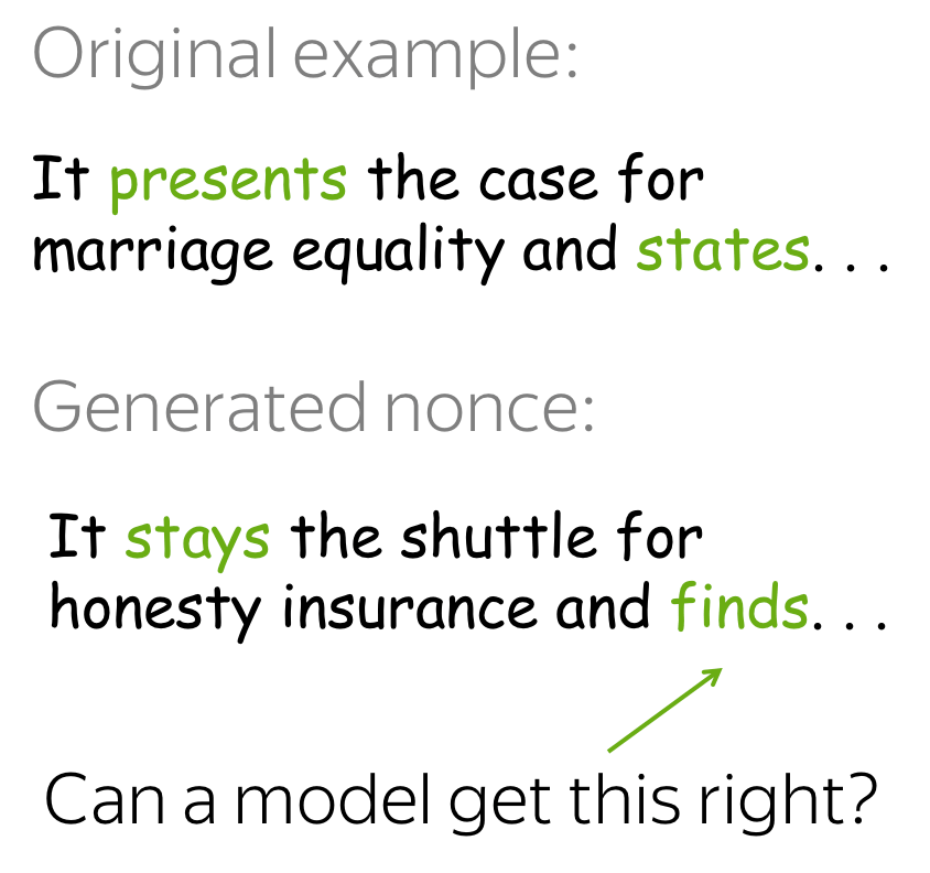
More details
How nonsense can help your research
To distinguish between cases where a model indeed learned grammatical agreement or just collocation, the authors test not only "normal" examples, but also the ones which do not make sense. E.g. does a model predict the correct agreement in the sentence The colorless green ideas I ate with the chair sleep furiously ?
The authors generate such examples: they take an original sentence and replace some words with random words, but preserving part-of-speech and morphological inflection. One example was shown above.
Look at the results ("5-gram KN" is the 5-gram model with Kneser-Ney smoothing).
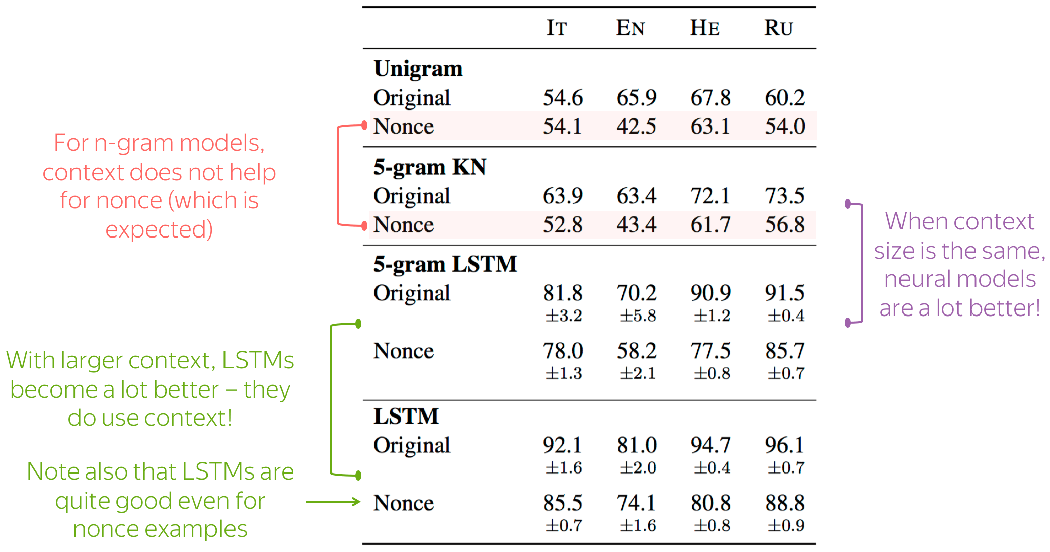
The results show that:
- for n-gram models, context does not help
For nonce sentences, 5-gram models are not better than unigram. A bit better for normal sentences though. - with the same context, LSTMs are a lot better than n-gram
The difference is huge for both original and nonce examples. This is the power of neural networks - they "know" which words are similar, while n-gram models rely only on co-occurrence.
Size is not the only thing that matters! Neural models are better not only because of context size but also because of how they process this context. - for LSTMs, large context does help
This is nice - it means that LSTMs do use long contexts. Note also that the scores are quite high even for nonce sentences!
More in the paper
- the detailed procedure for generating nonce examples;
- results and discussion for specific grammatical constructions.
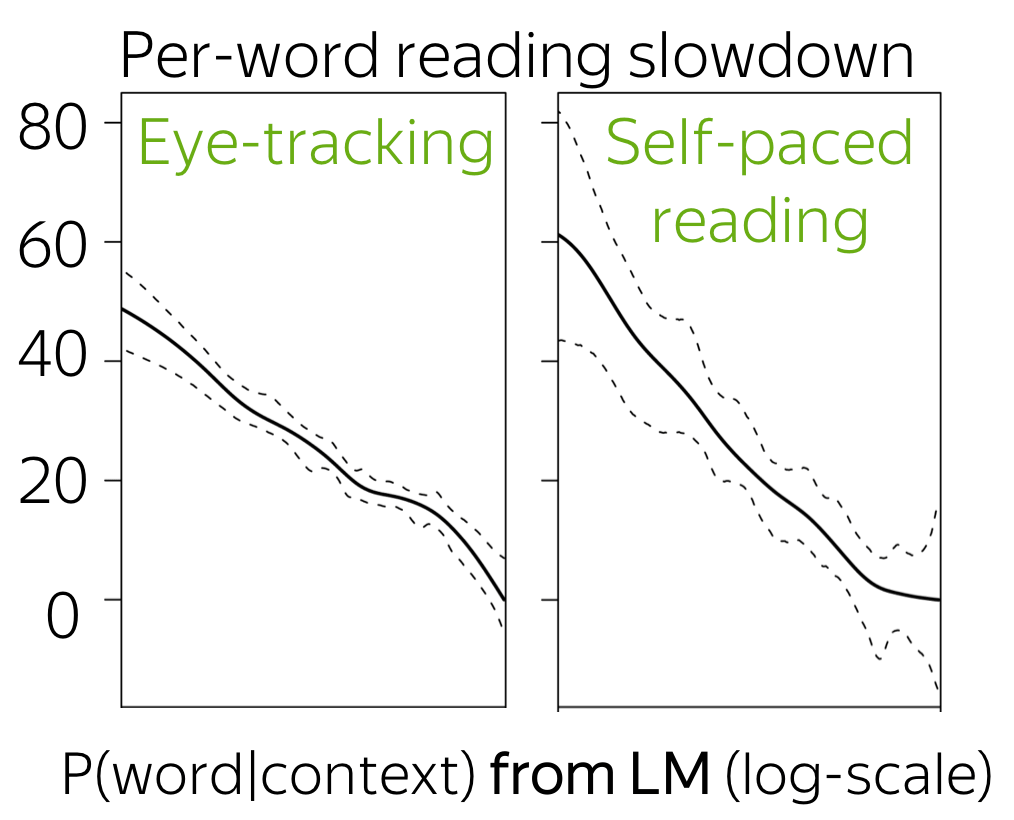
Language Models and Human Reading Behavior
Lena: This is not what you will typically see at the "Related Papers" lists for a language modeling lecture (at least, I never saw in any). But when I first found this, I was so excited, that I can't help sharing it with you :)
The time it takes humans to read a word can be predicted from estimates of the word's probability in context. The paper shows that (i) P(word|context) from an n-gram language model is a very good predictor of this time; (ii) the relationship between word log-probability and reading time is (near-)linear (see the figure).
More details
Time to read vs Predictability of a word in the context
When we read a text, the time taken to read each word is related to our expectations about this word: the more "expected" a word is, the less time we need to read it. However, the exact functional relation between this per-word processing time in humans and the "predictability" of a word given context was not known.
The key point of this paper is that a language model can be used to estimate the "predictability" of a word given context.
Computational LM instead of a Human one - a very novel idea
Previously, the predictability of a word given context was estimated in cloze-style tasks: humans were asked to guess the next word given context. For example, to continue the sentences
(1) My brother came inside to...
(2) The children went outside to...
In the first case, the continuation can be very different, but in the second case, about 90% of participants suggest the word play.
While this data estimates the word predictability directly, it is very sparse: for most of the continuations, there's no data at all. That's why the idea to use a computational language model instead of a human one was so groundbreaking: it allowed to estimate word predictability very easily.
Components of the study
Data with human behavior:
- eye-tracking
Eye movements of native speakers reading a newspaper text. - self-paced reading
Moving-window self-paced reading times: the participant must press a button to reveal each word in turn. Data recorded: the times between button presses.
Language model: 3-gram with Kneser-Ney smoothing.
Results
- computational language models can be very good at predicting time taken by humans to read a word;
- the functional relationship between reading time and predictability is now known: it is logarithmic (i.e., the relationship between word log-probability and reading time is (near-)linear - this is what we see on the figure).
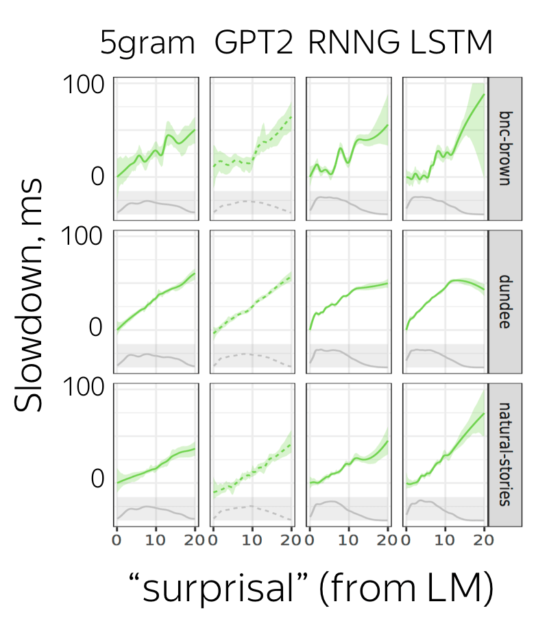
In light of the previous work, explore which LMs (across architectures and datasets) are better at predicting human behavior. Overall, the traditional LM perplexity is a good estimate of this. Strangely, Transformers (which we'll meet at the next lecture) and n-gram LMs are better than LSTMs.
More details
Considered models
- 5-gram: 5-gram LM with Kneser-Ney smoothing;
- LSTM: the standard ones;
- RNNG: models the joint probability of a sequence of words as well as its syntactic structure;
- GPT-2: Transformer LM. This a very popular model which we'll meet a bit later in the course.
LM Surprisal vs Reading Times
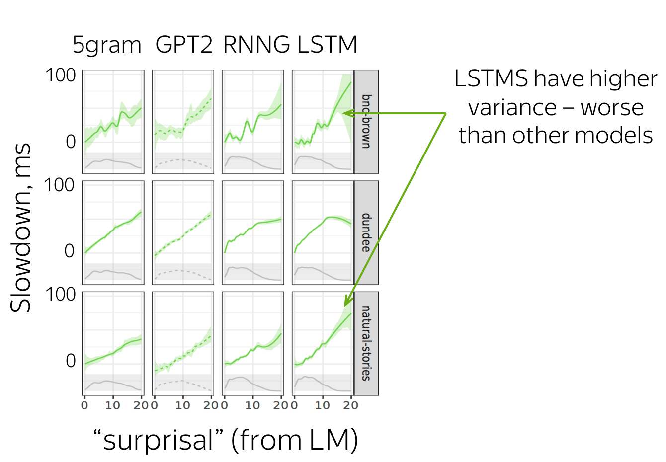
The figure shows the relationship between LM "surprisals" (negative log-probability) and human reading times for all models and corpora (more in the original paper!). Main observations are:
- the relationship is linear for all models;
- human reading time has higher variance with respect to LSTM predictions than with respect to predictions of other models.
Psychometric Predictive Power vs LM Perplexity
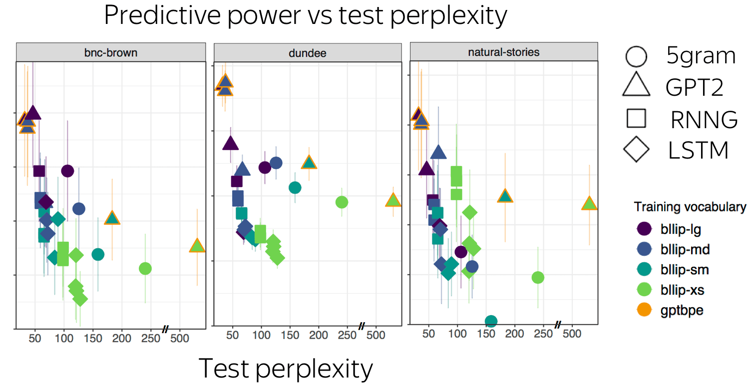
(The scary phrase "psychometric predictive power" simply means how good is an LM at predicting human behavior.)
Generally, we see that models with lower perplexity (in NLP, we think are good models) are also good at predicting human behavior.
N-gram LMs: More Smoothings
Kneser-Ney Smoothing
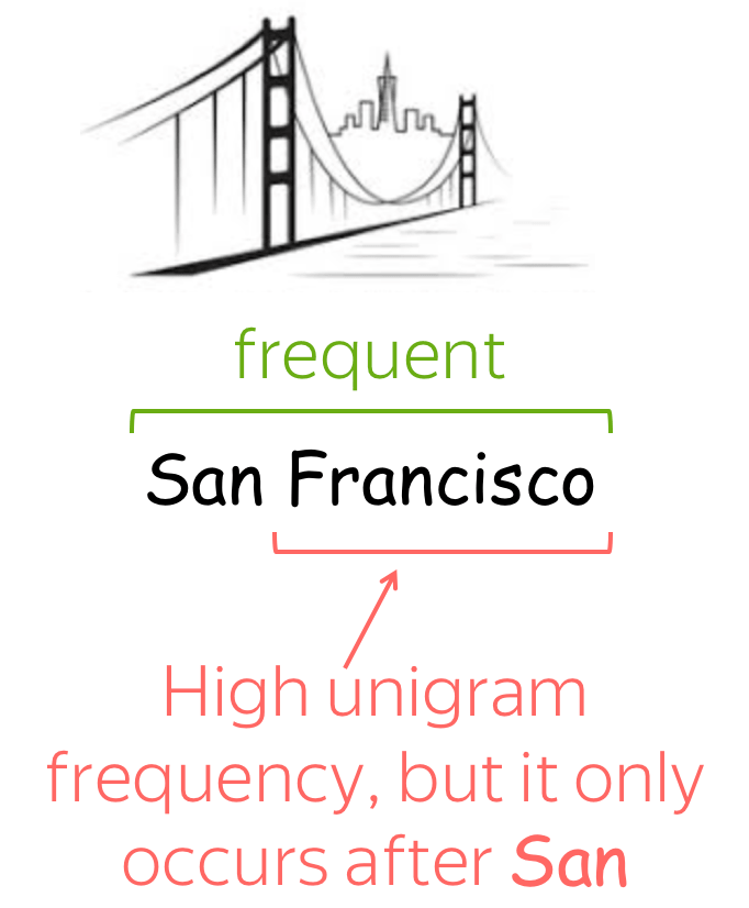
Simple back-off smoothings discard context and back off from n-grams to k-grams with k < n. But let's take for example a phrase San Francisco: it is common and Francisco will have a high unigram probability. And here's the problem: Francisco appears mostly after San, but when backing off, it's large unigram probability will result in a large probability of Francisco after any token!
More details
Unigram Probability: Stupid Back-off vs Kneser-Ney
Before looking at the full Kneser-Ney formula, let's first compare the unigram probabilities for a token which uses Kneser-Ney and stupid back-off smoothings. Stupid Back-off is based on simple unigram counts \(N(w_i)\): the number of times \(w_i\) occurs in the corpus. As we mentioned earlier, this won't work well for examples like San Francisco.
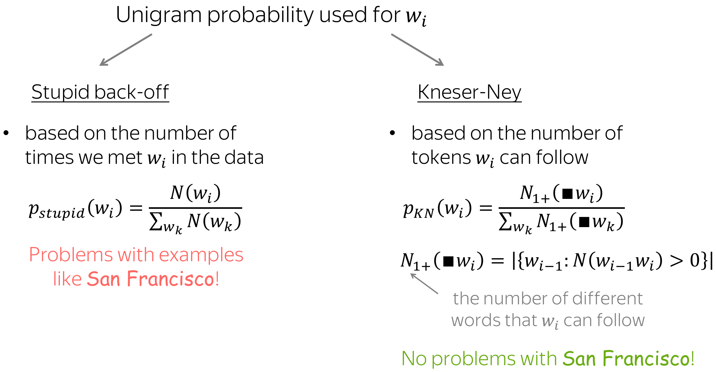
In contrast to simple back-off, Kneser-Ney smoothing uses not the raw counts, but the number of tokens \(w_i\) can follow. Intuitively, this is exactly what we want: we need something which tells us how likely \(w_i\) can continue a prefix. In our example, Francisco will get low probability (just as it should).
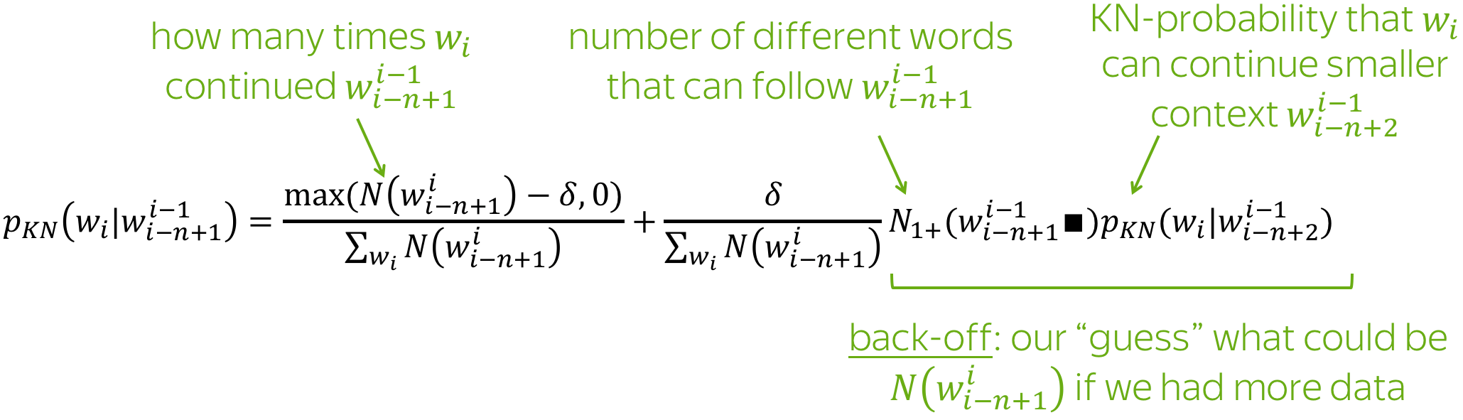
Going Further: Iterative Formula
For the full formula, we need to define one more count:

The full back-off formula for Kneser-Ney is shown below.
Here will be more papers!
The papers will be gradually appearing.

Have Fun!
Let's write a paper!
Every great paper starts with an inciting thought - something only a human can have ...
Waiting for the model to load... (this should take 3-5s)