Word Embeddings
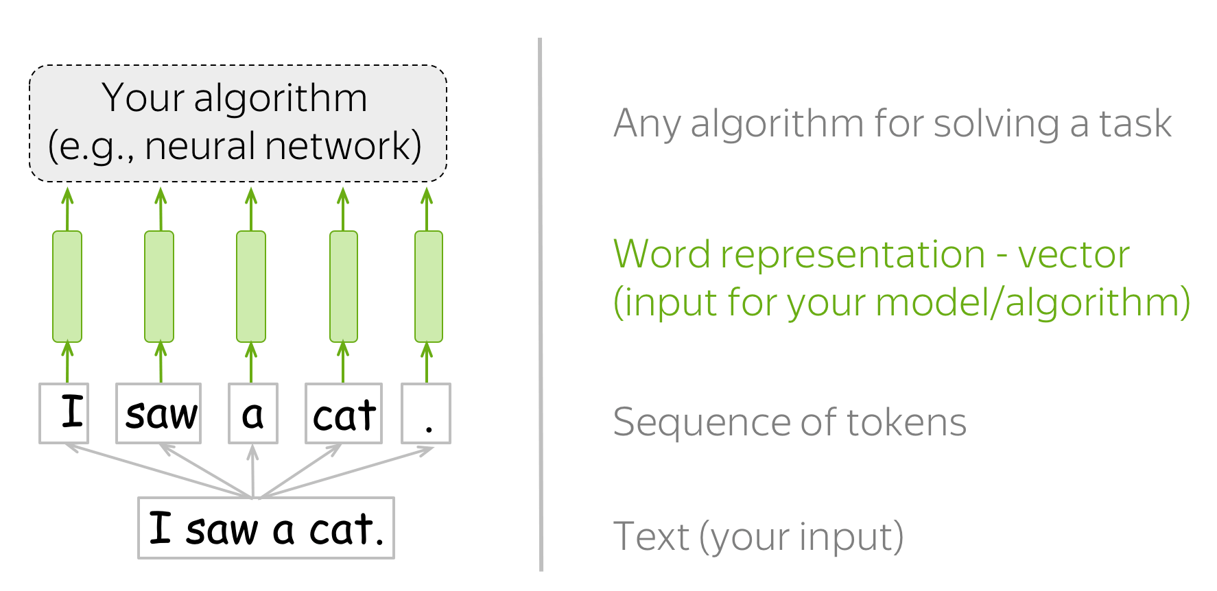
The way machine learning models "see" data is different from how we (humans) do. For example, we can easily understand the text "I saw a cat", but our models can not - they need vectors of features. Such vectors, or word embeddings, are representations of words which can be fed into your model.
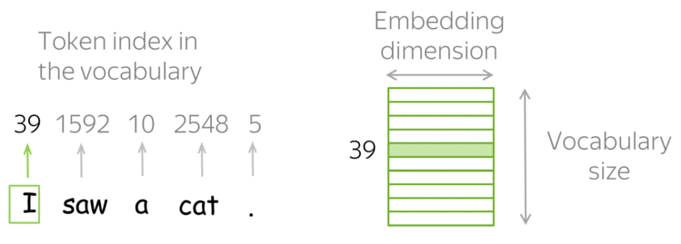
How it works: Look-up Table (Vocabulary)
In practice, you have a vocabulary of allowed words; you choose this vocabulary in advance. For each vocabulary word, a look-up table contains its embedding. This embedding can be found using the word index in the vocabulary (i.e., you to look up the embedding in the table using word index).
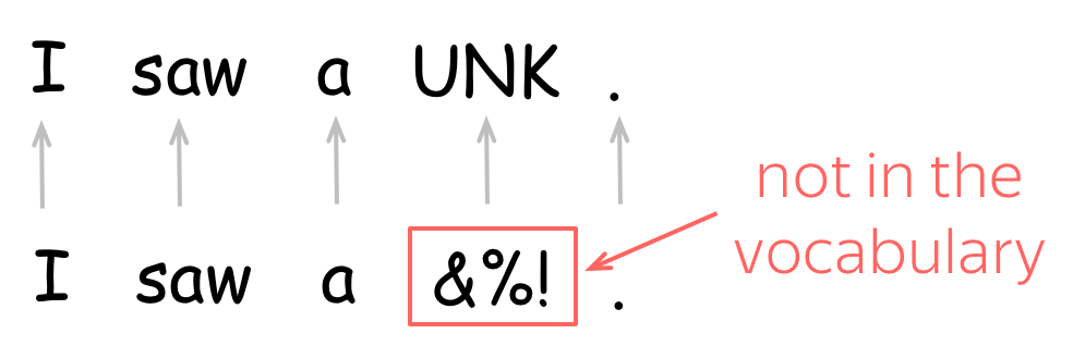
To account for unknown words (the ones which are not in the vocabulary), usually a vocabulary contains a special token UNK. Alternatively, unknown tokens can be ignored or assigned a zero vector.
The main question of this lecture is: how do we get these word vectors?
Represent as Discrete Symbols: One-hot Vectors
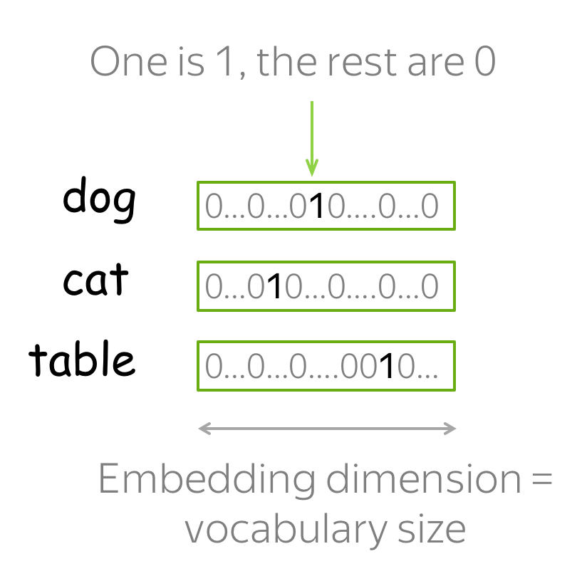
The easiest you can do is to represent words as one-hot vectors: for the i-th word in the vocabulary, the vector has 1 on the i-th dimension and 0 on the rest. In Machine Learning, this is the most simple way to represent categorical features.
You probably can guess why one-hot vectors are not the best way to represent words. One of the problems is that for large vocabularies, these vectors will be very long: vector dimensionality is equal to the vocabulary size. This is undesirable in practice, but this problem is not the most crucial one.
What is really important, is that these vectors know nothing about the words they represent. For example, one-hot vectors "think" that cat is as close to dog as it is to table! We can say that one-hot vectors do not capture meaning.
But how do we know what is meaning?
Distributional Semantics
To capture meaning of words in their vectors, we first need to define the notion of meaning that can be used in practice. For this, let us try to understand how we, humans, get to know which words have similar meaning.
How to: go over the slides at your pace. Try to notice how your brain works.
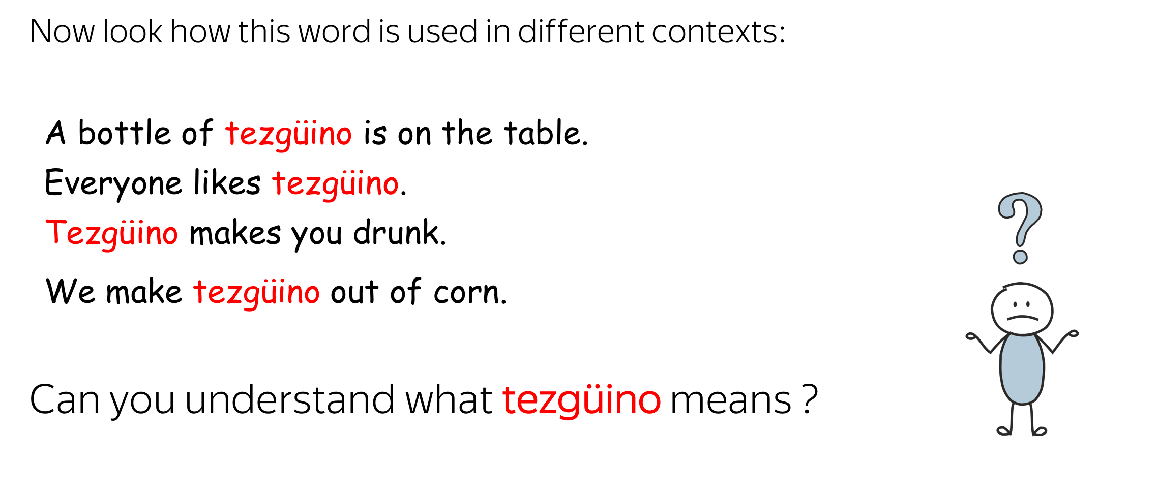
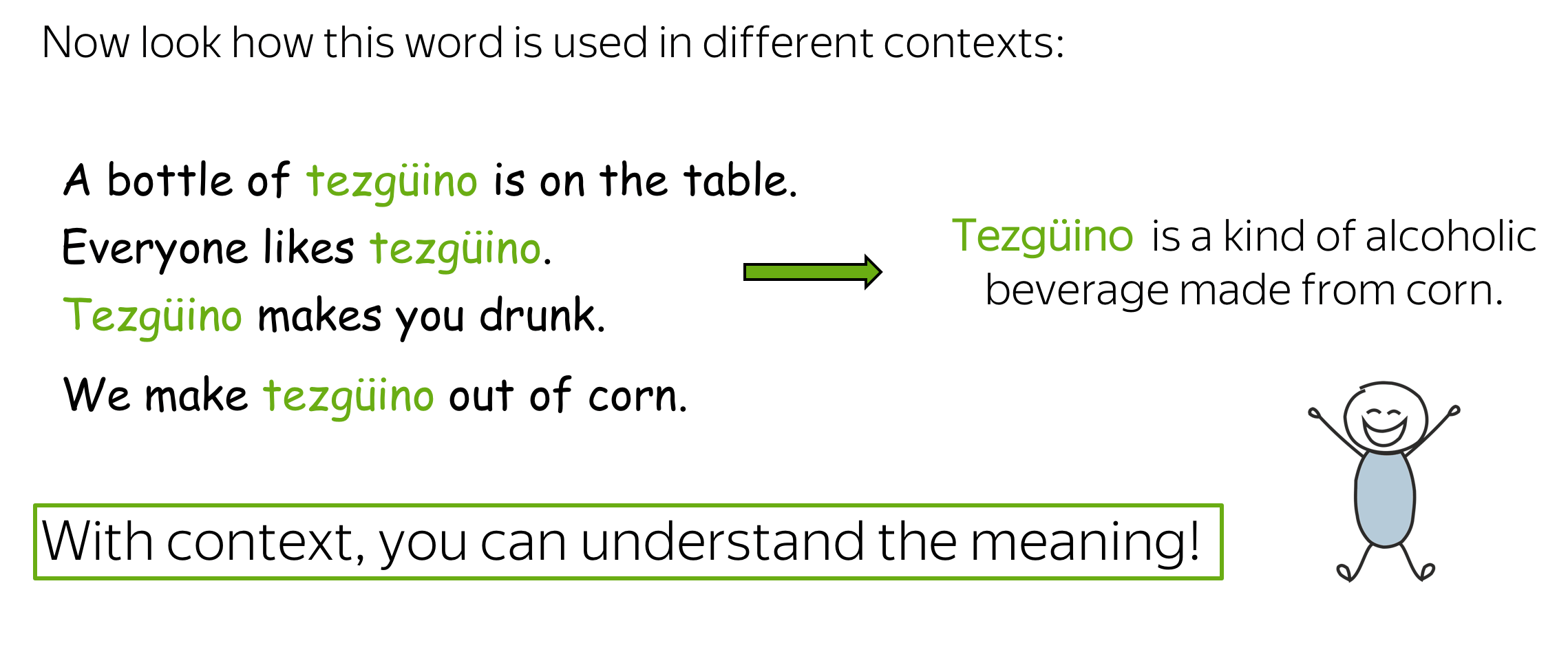
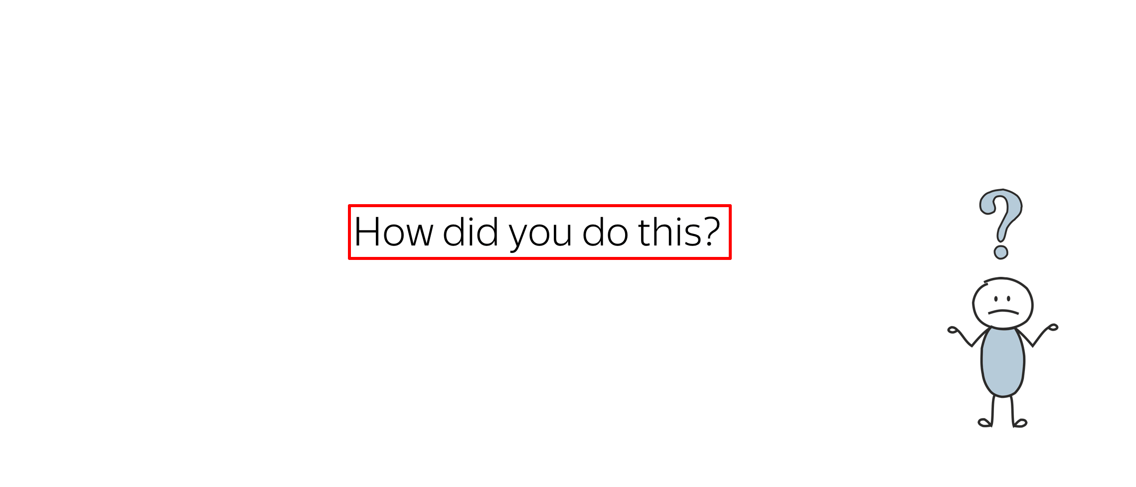
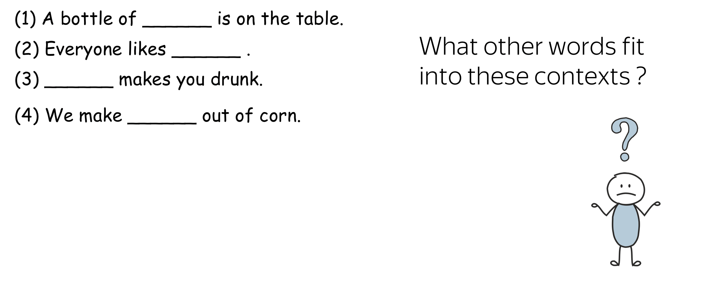
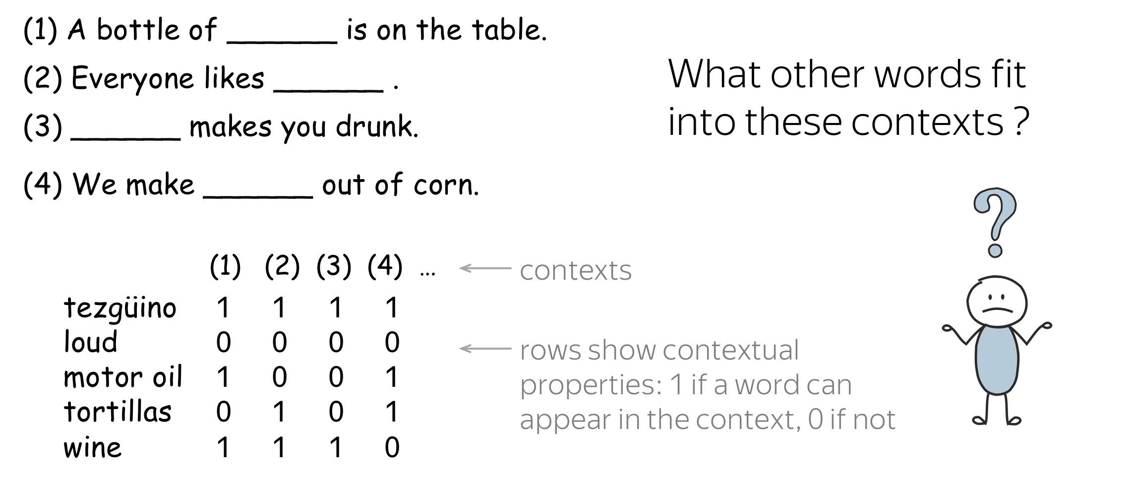
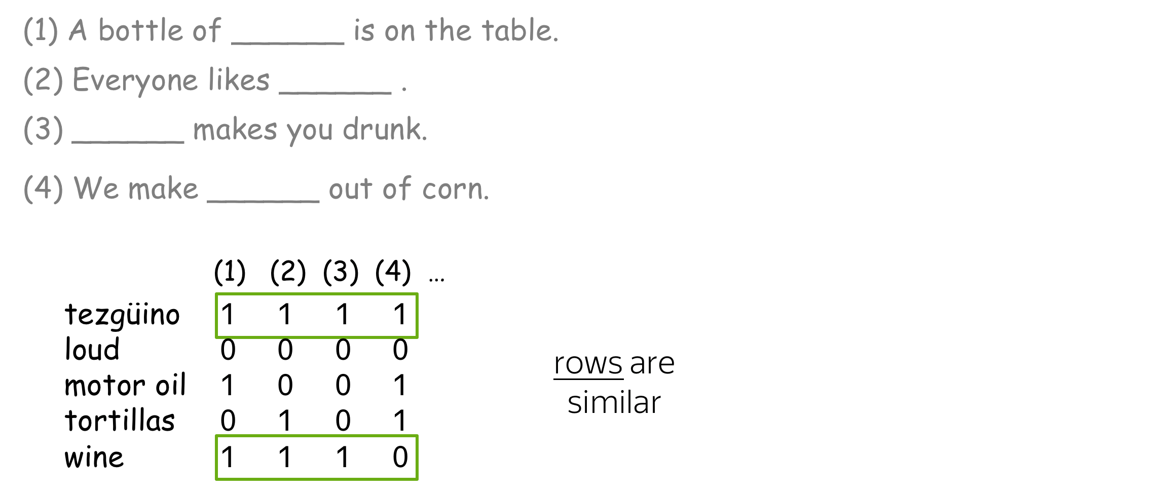
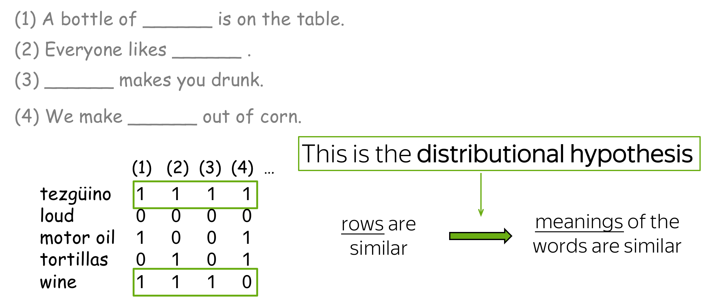
Once you saw how the unknown word used in different contexts, you were able to understand it's meaning. How did you do this?
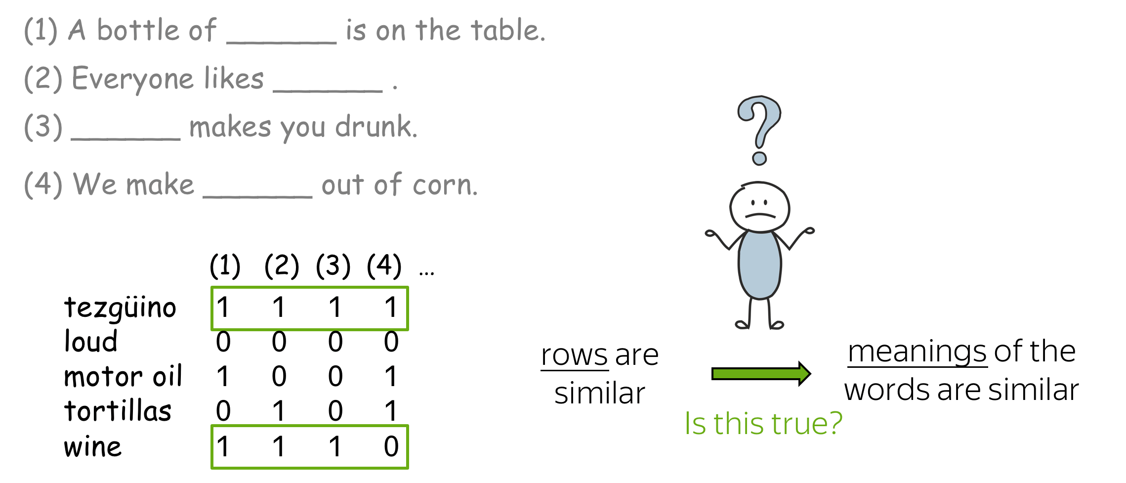
The hypothesis is that your brain searched for other words that can be used in the same contexts, found some (e.g., wine), and made a conclusion that tezgüino has meaning similar to those other words. This is the distributional hypothesis:
Words which frequently appear in similar contexts have similar meaning.
Lena: Often you can find it formulated as "You shall know a word by the company it keeps" with the reference to J. R. Firth in 1957, but actually there were a lot more people responsible, and much earlier. For example, Harris, 1954.
This is an extremely valuable idea: it can be used in practice to make word vectors capture their meaning. According to the distributional hypothesis, "to capture meaning" and "to capture contexts" are inherently the same. Therefore, all we need to do is to put information about word contexts into word representation.
Main idea: We need to put information about word contexts into word representation.
All we'll be doing at this lecture is looking at different ways to do this.
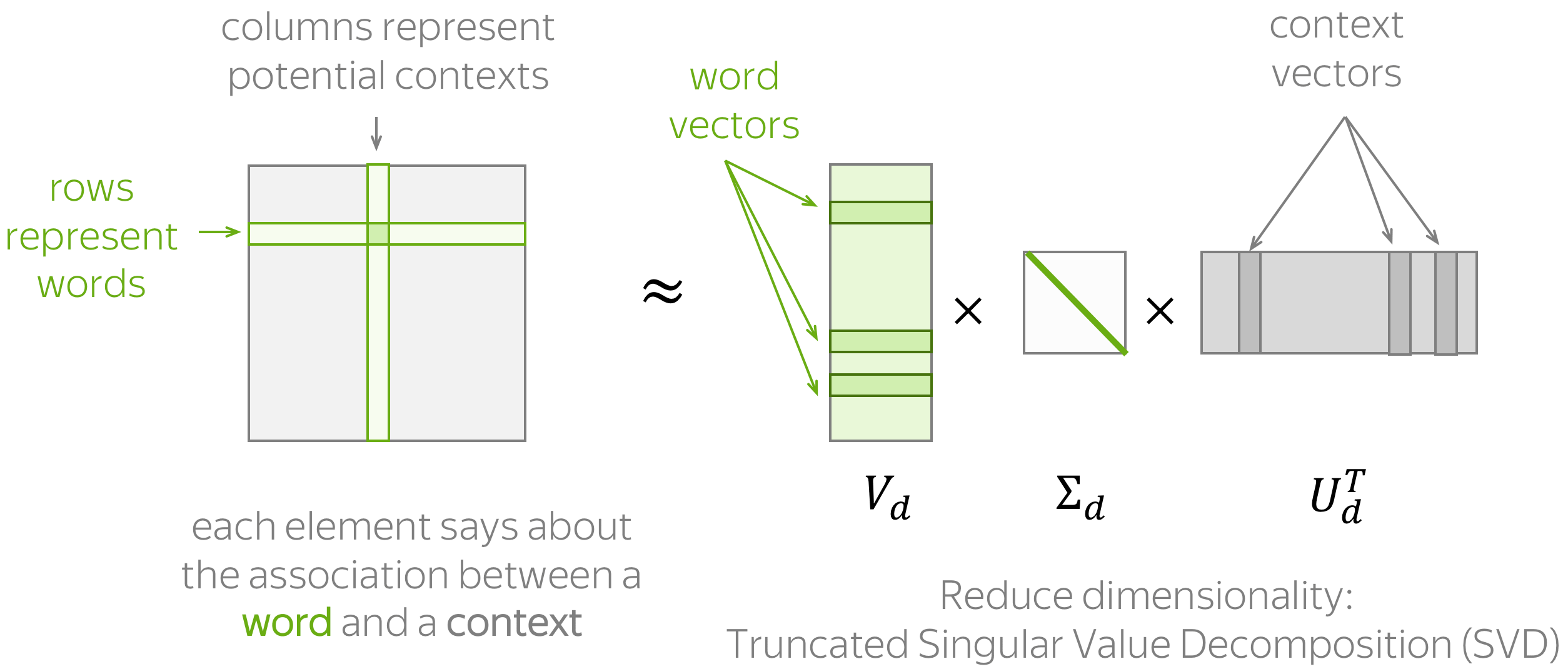
Count-Based Methods
Let's remember our main idea:
Main idea: We have to put information about contexts into word vectors.
Count-based methods take this idea quite literally:
How: Put this information manually based on global corpus statistics.
The general procedure is illustrated above and consists of the two steps: (1) construct a word-context matrix, (2) reduce its dimensionality. There are two reasons to reduce dimensionality. First, a raw matrix is very large. Second, since a lot of words appear in only a few of possible contexts, this matrix potentially has a lot of uninformative elements (e.g., zeros).
To estimate similarity between words/contexts, usually you need to evaluate the dot-product of normalized word/context vectors (i.e., cosine similarity).
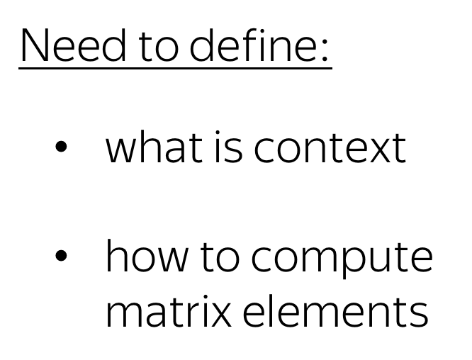
To define a count-based method, we need to define two things:
- possible contexts (including what does it mean that a word appears in a context),
- the notion of association, i.e., formulas for computing matrix elements.
Below we provide a couple of popular ways of doing this.
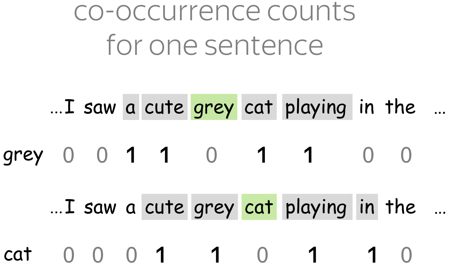
Simple: Co-Occurence Counts
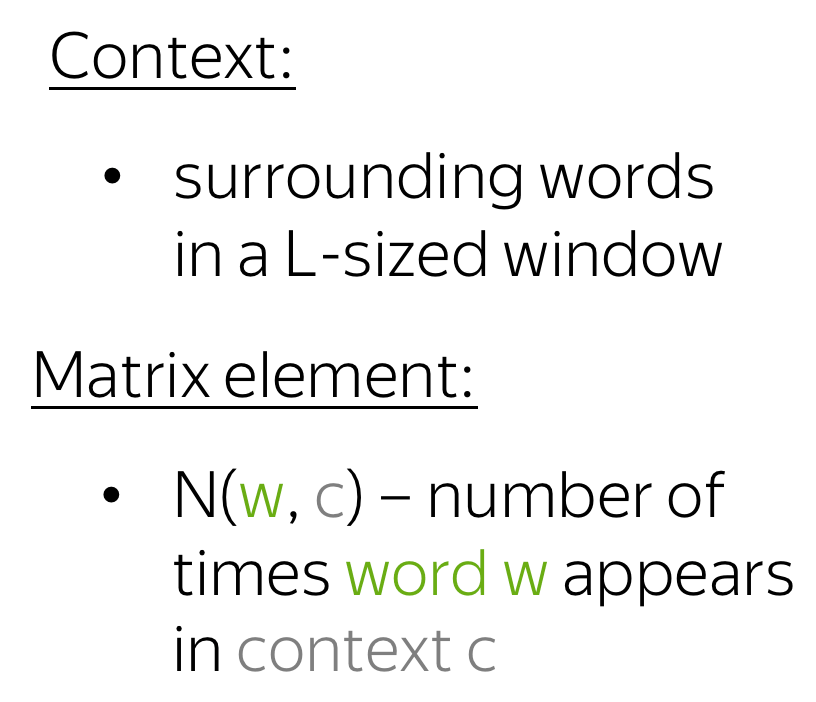
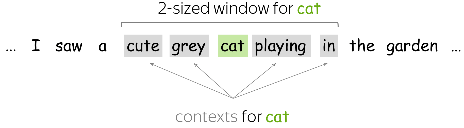
The simplest approach is to define contexts as each word in an L-sized window. Matrix element for a word-context pair (w, c) is the number of times w appears in context c. This is the very basic (and very, very old) method for obtaining embeddings.
The (once) famous HAL model (1996) is also a modification of this approach. Learn more from this exercise in the Research Thinking section.
Positive Pointwise Mutual Information (PPMI)
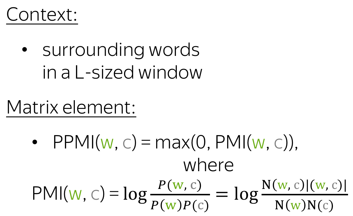
Here contexts are defined as before, but the measure of the association between word and context is more clever: positive PMI (or PPMI for short). PPMI measure is widely regarded as state-of-the-art for pre-neural distributional-similarity models.
Important: relation to neural models!
Turns out, some of the neural methods we will consider (Word2Vec) were shown
to implicitly approximate the factorization of a (shifted) PMI matrix. Stay tuned!
Latent Semantic Analysis (LSA): Understanding Documents
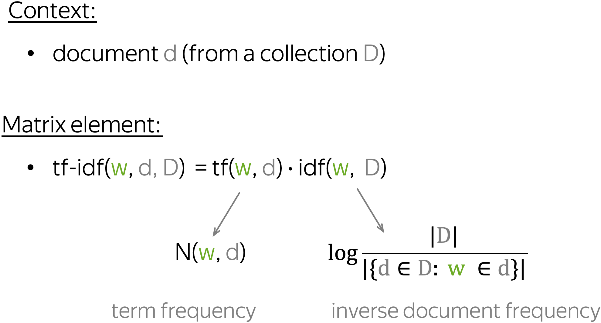
Latent Semantic Analysis (LSA) analyzes a collection of documents. While in the previous approaches contexts served only to get word vectors and were thrown away afterward, here we are also interested in context, or, in this case, document vectors. LSA is one of the simplest topic models: cosine similarity between document vectors can be used to measure similarity between documents.
The term "LSA" sometimes refers to a more general approach of applying SVD to a term-document matrix where the term-document elements can be computed in different ways (e.g., simple co-occurrence, tf-idf, or some other weighting).
Animation alert! LSA wikipedia page has a nice animation of the topic detection process in a document-word matrix - take a look!
Word2Vec: a Prediction-Based Method
Let us remember our main idea again:
Main idea: We have to put information about contexts into word vectors.
While count-based methods took this idea quite literally, Word2Vec uses it in a different manner:
How: Learn word vectors by teaching them to predict contexts.
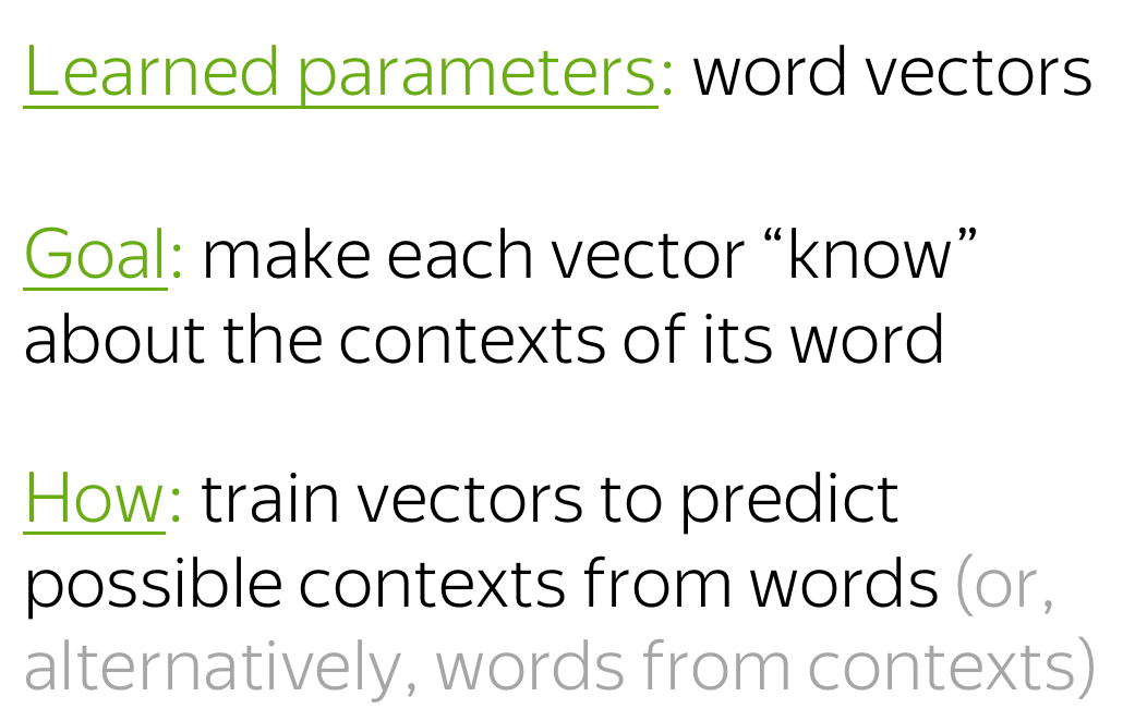
Word2Vec is a model whose parameters are word vectors. These parameters are optimized iteratively for a certain objective. The objective forces word vectors to "know" contexts a word can appear in: the vectors are trained to predict possible contexts of the corresponding words. As you remember from the distributional hypothesis, if vectors "know" about contexts, they "know" word meaning.
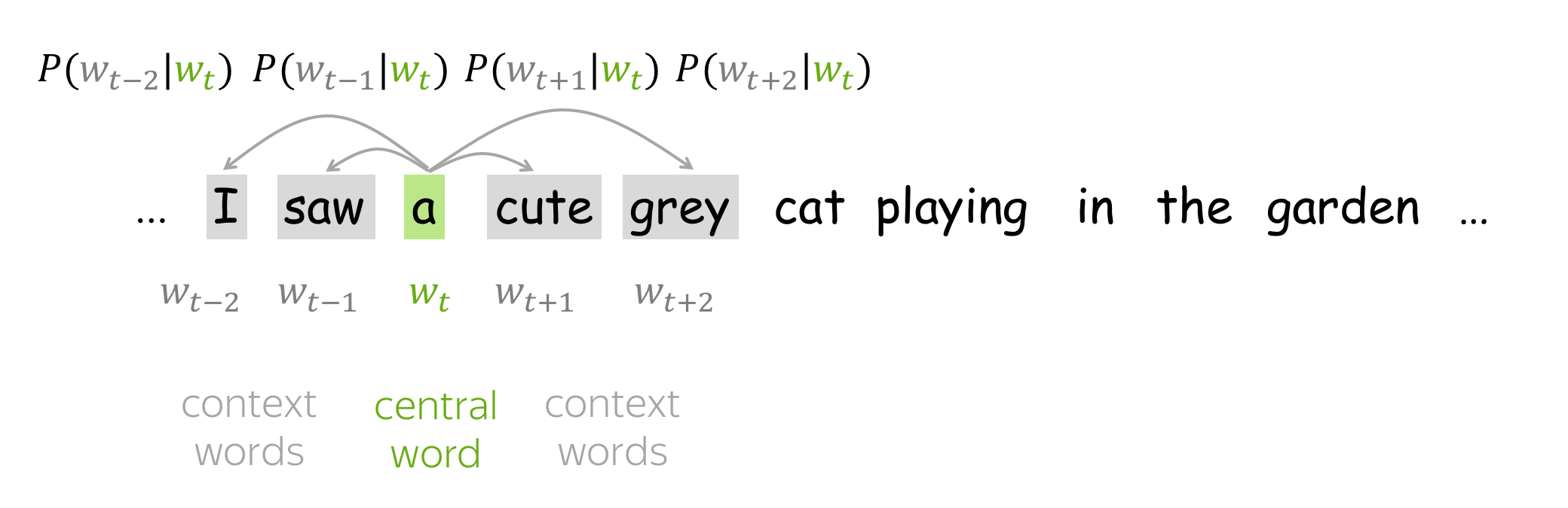
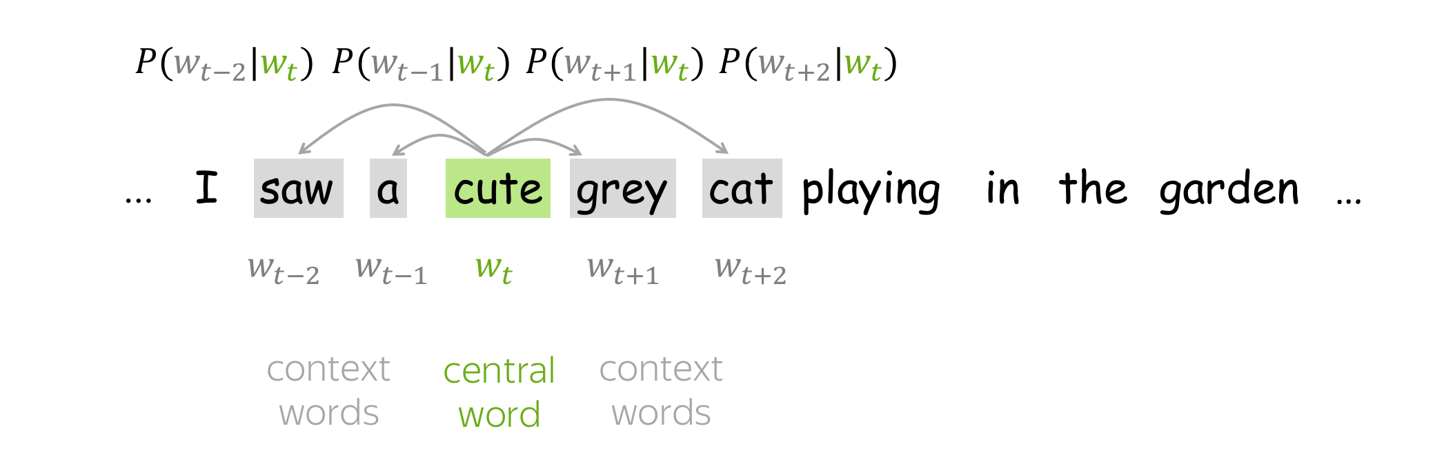
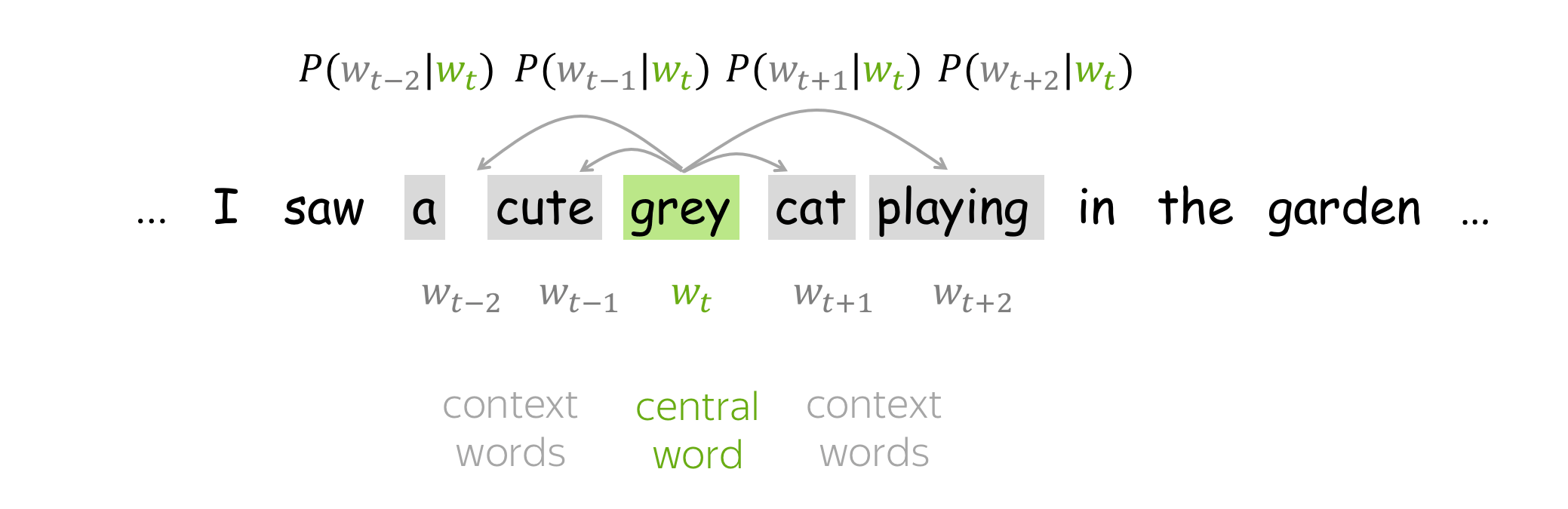
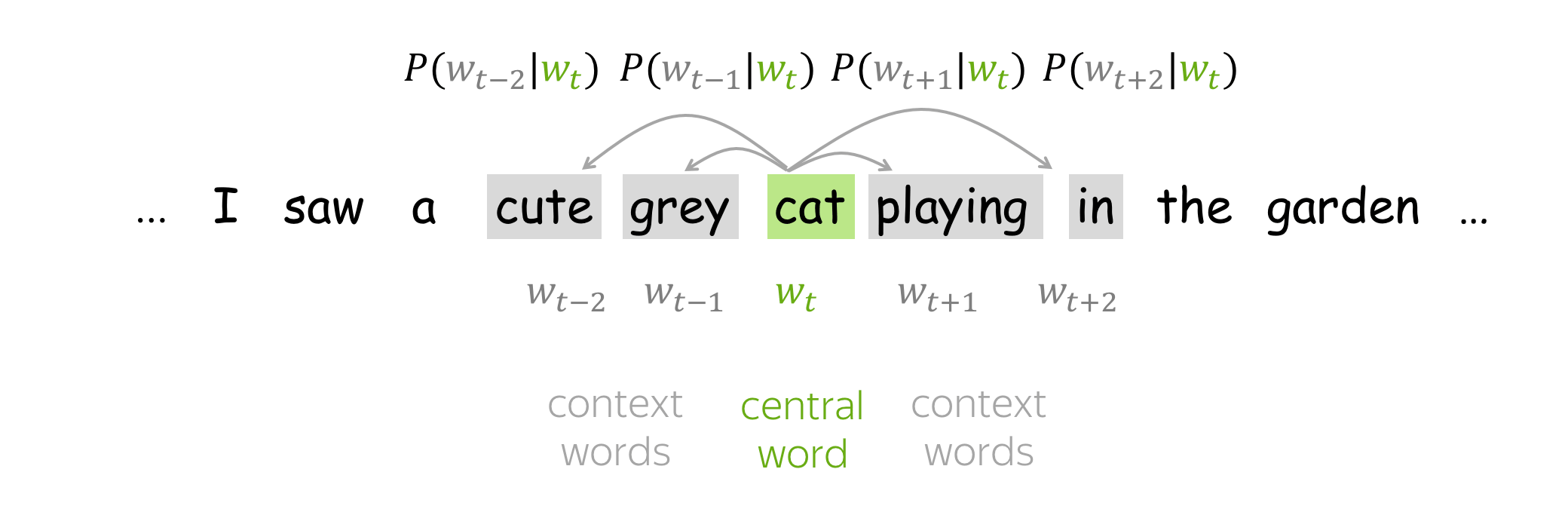
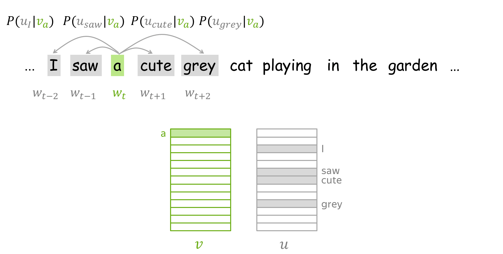
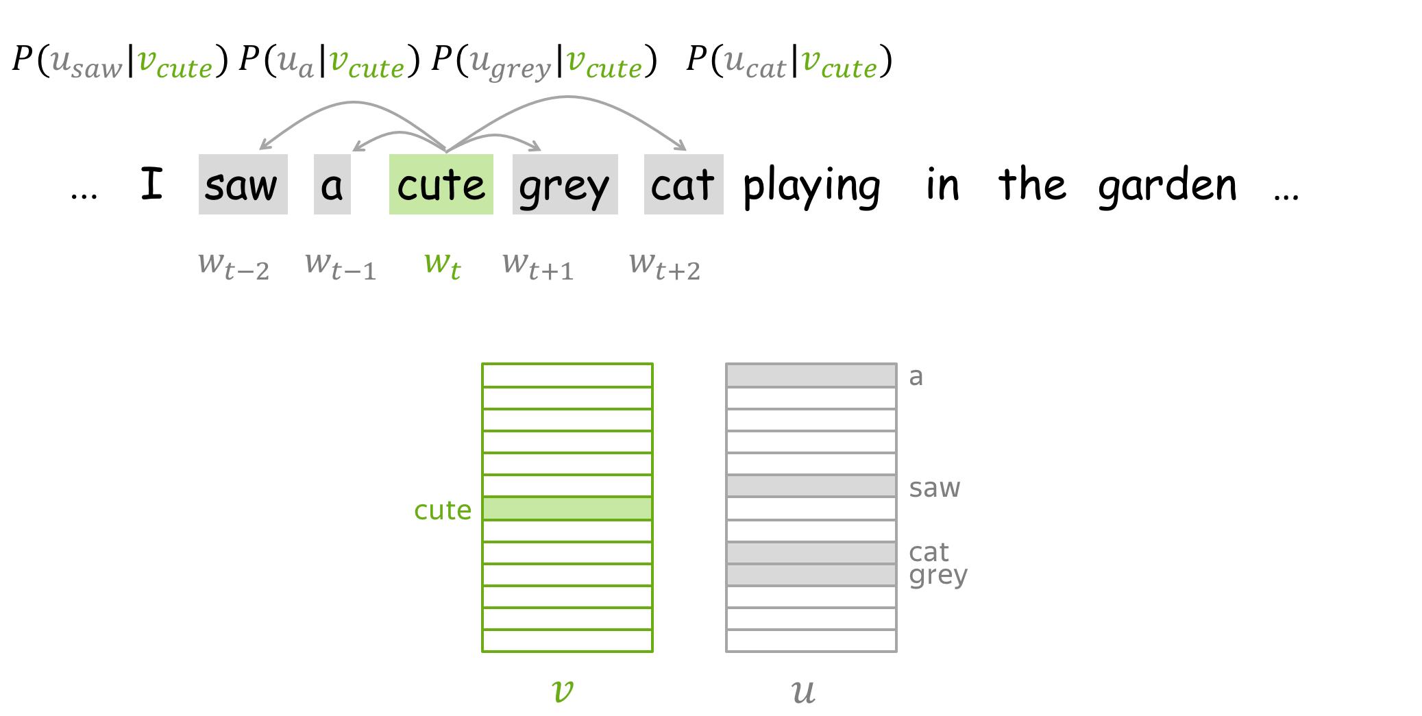
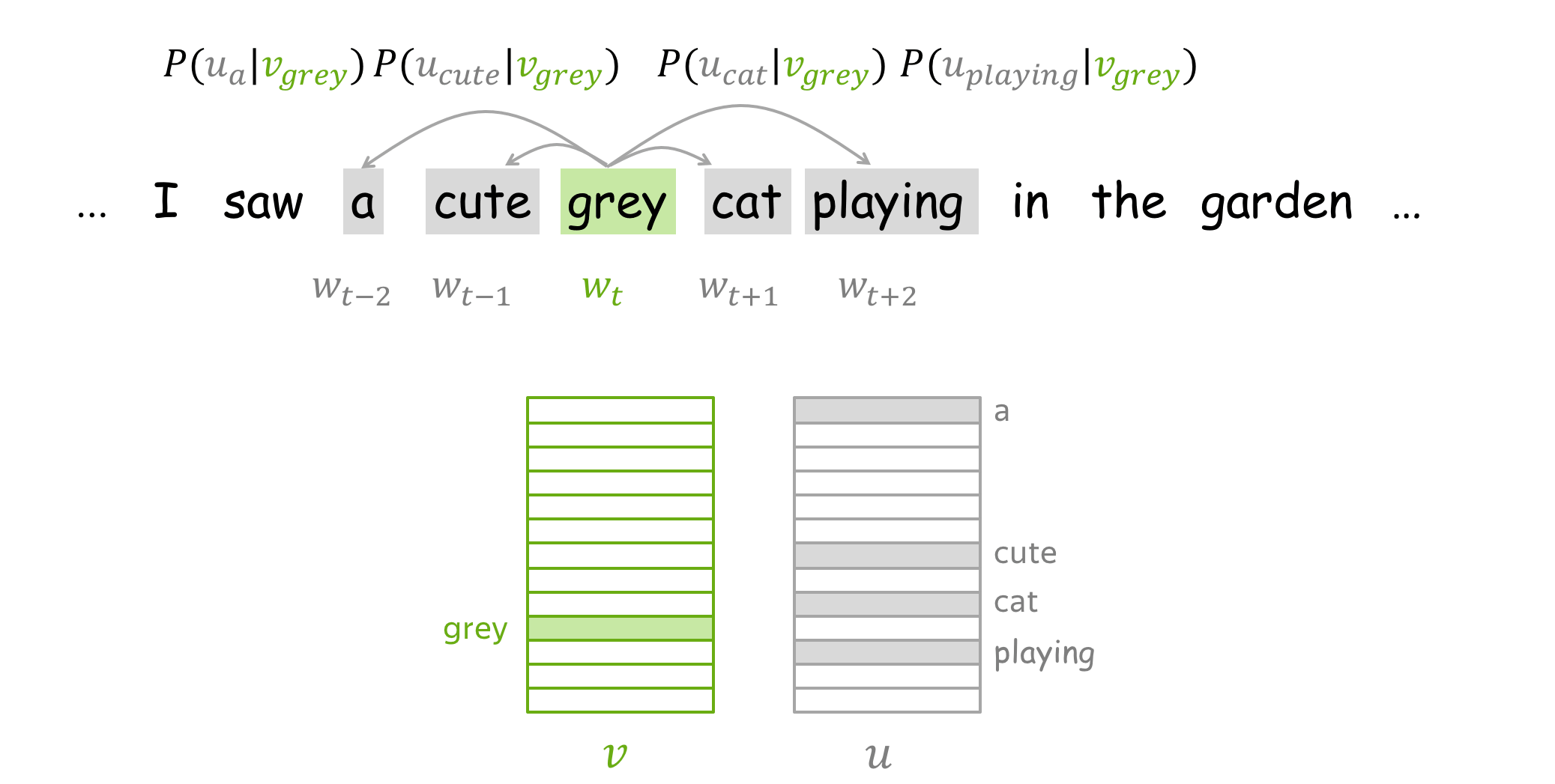
Word2Vec is an iterative method. Its main idea is as follows:
- take a huge text corpus;
- go over the text with a sliding window, moving one word at a time. At each step, there is a central word and context words (other words in this window);
- for the central word, compute probabilities of context words;
- adjust the vectors to increase these probabilities.
How to: go over the illustration to understand the main idea.
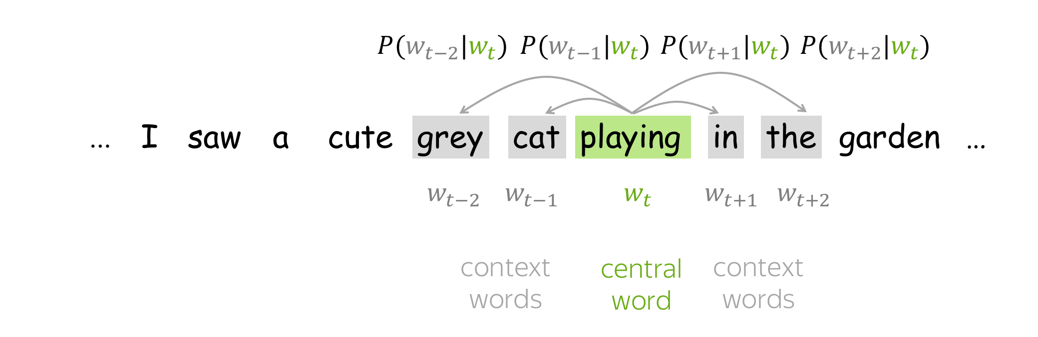
Lena: Visualization idea is from the Stanford CS224n course.
Objective Function: Negative Log-Likelihood
For each position \(t =1, \dots, T\) in a text corpus, Word2Vec predicts context words within a m-sized window given the central word \(\color{#88bd33}{w_t}\): \[\color{#88bd33}{\mbox{Likelihood}} \color{black}= L(\theta)= \prod\limits_{t=1}^T\prod\limits_{-m\le j \le m, j\neq 0}P(\color{#888}{w_{t+j}}|\color{#88bd33}{w_t}\color{black}, \theta), \] where \(\theta\) are all variables to be optimized. The objective function (aka loss function or cost function) \(J(\theta)\) is the average negative log-likelihood:
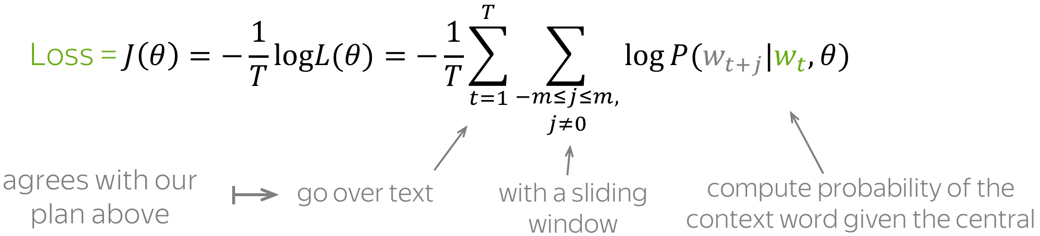
Note how well the loss agrees with our plan main above: go over text with a sliding window and compute probabilities. Now let's find out how to compute these probabilities.
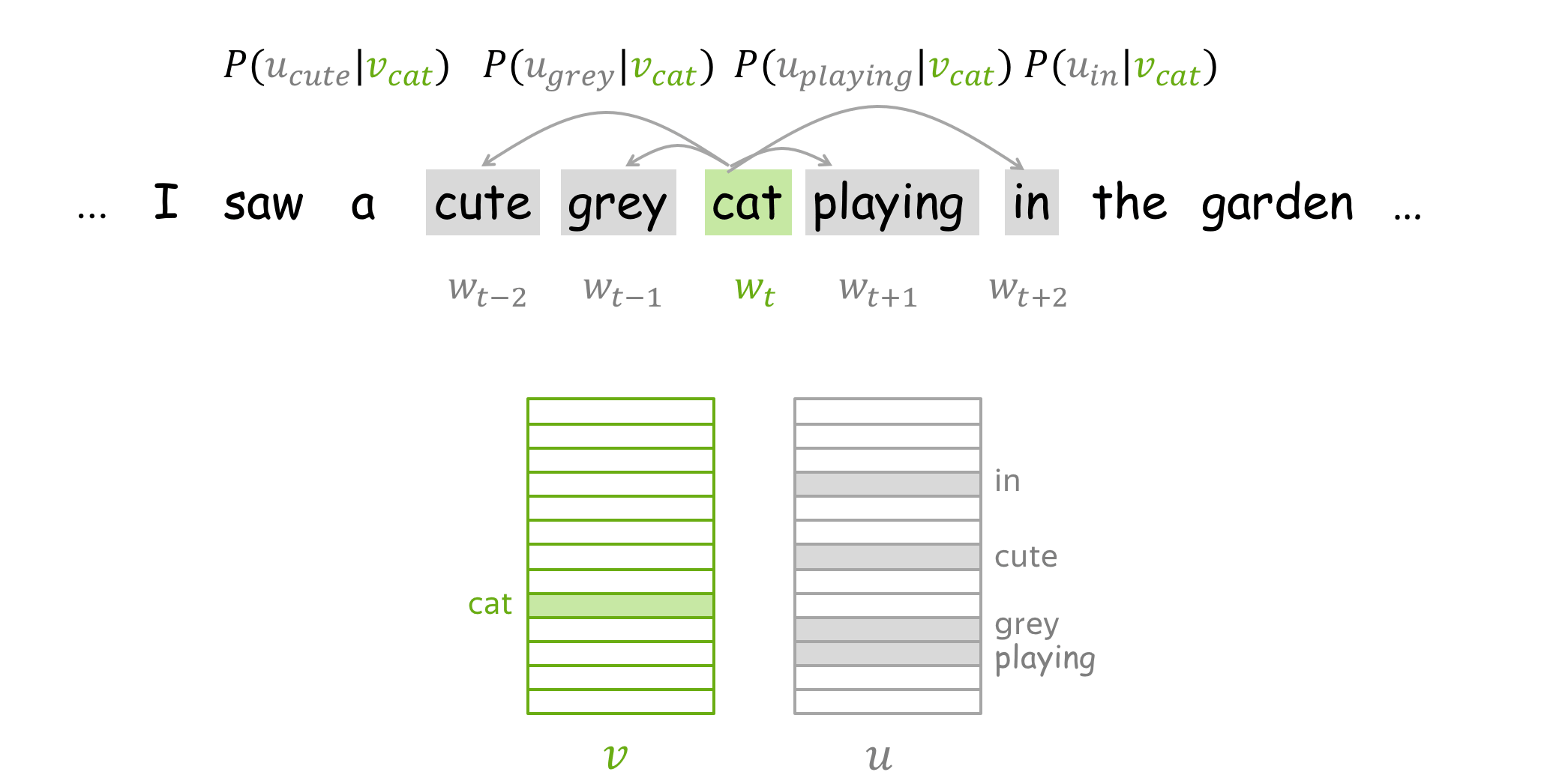
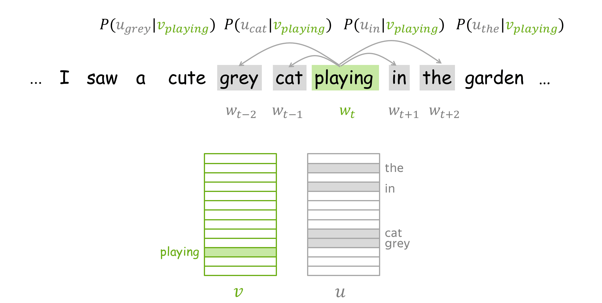
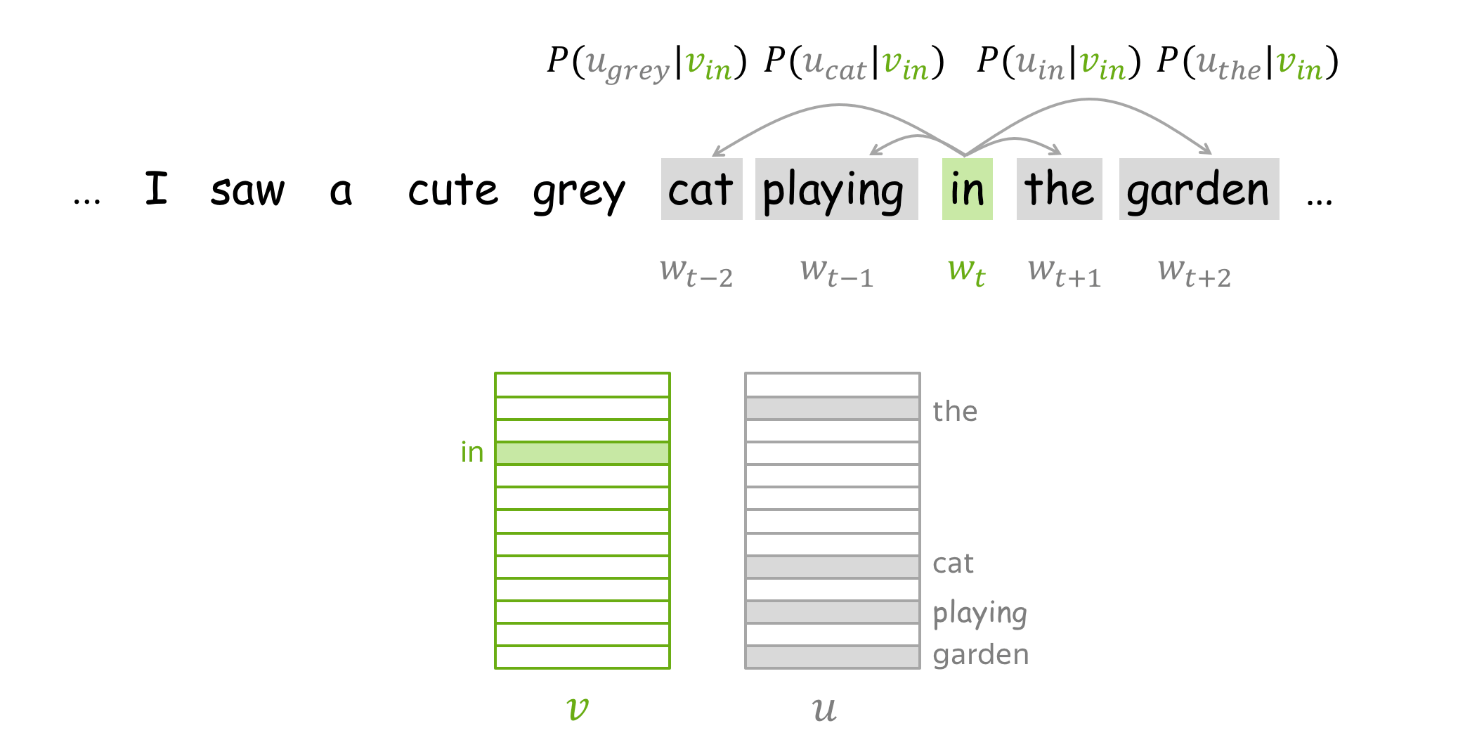
How to calculate \(P(\color{#888}{w_{t+j}}\color{black}|\color{#88bd33}{w_t}\color{black}, \theta)\)?
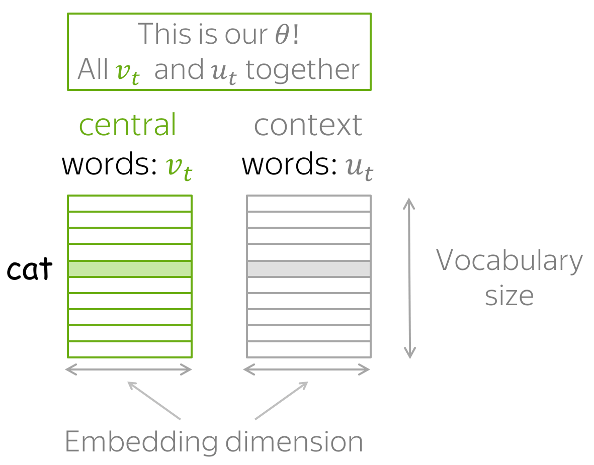
For each word \(w\) we will have two vectors:
- \(\color{#88bd33}{v_w}\) when it is a central word;
- \(\color{#888}{u_w}\) when it is a context word.
(Once the vectors are trained, usually we throw away context vectors and use only word vectors.)
Then for the central word \(\color{#88bd33}{c}\) (c - central) and the context word \(\color{#888}{o}\) (o - outside word) probability of the context word is
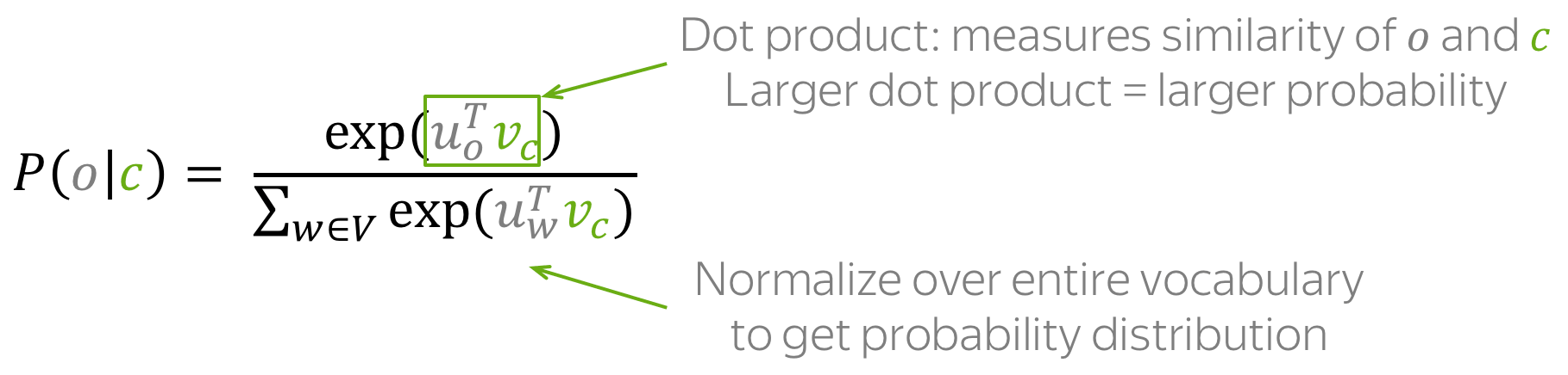
Note: this is the softmax function! (click for the details)
The function above is an example of the softmax function: \[softmax(x_i)=\frac{\exp(x_i)}{\sum\limits_{j=i}^n\exp(x_j)}.\] Softmax maps arbitrary values \(x_i\) to a probability distribution \(p_i\):
- "max" because the largest \(x_i\) will have the largest probability \(p_i\);
- "soft" because all probabilities are non-zero.
You will deal with this function quite a lot over the NLP course (and in Deep Learning in general).
How to: go over the illustration. Note that for central words and context words, different vectors are used. For example, first the word a is central and we use \(\color{#88bd33}{v_a}\), but when it becomes context, we use \(\color{#888}{u_a}\) instead.
How to train: by Gradient Descent, One Word at a Time
Let us recall that our parameters \(\theta\) are vectors \(\color{#88bd33}{v_w}\) and \(\color{#888}{u_w}\) for all words in the vocabulary. These vectors are learned by optimizing the training objective via gradient descent (with some learning rate \(\alpha\)): \[\theta^{new} = \theta^{old} - \alpha \nabla_{\theta} J(\theta).\]
One word at a time
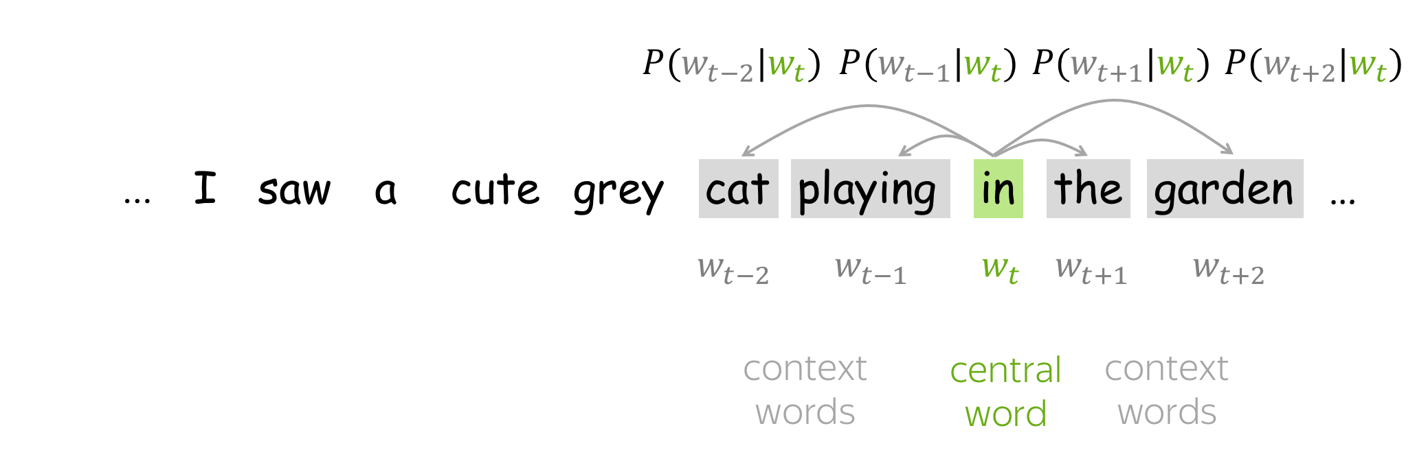
We make these updates one at a time: each update is for a single pair of a center word and one of its context words. Look again at the loss function: \[\color{#88bd33}{\mbox{Loss}}\color{black} =J(\theta)= -\frac{1}{T}\log L(\theta)= -\frac{1}{T}\sum\limits_{t=1}^T \sum\limits_{-m\le j \le m, j\neq 0}\log P(\color{#888}{w_{t+j}}\color{black}|\color{#88bd33}{w_t}\color{black}, \theta)= \frac{1}{T} \sum\limits_{t=1}^T \sum\limits_{-m\le j \le m, j\neq 0} J_{t,j}(\theta). \] For the center word \(\color{#88bd33}{w_t}\), the loss contains a distinct term \(J_{t,j}(\theta)=-\log P(\color{#888}{w_{t+j}}\color{black}|\color{#88bd33}{w_t}\color{black}, \theta)\) for each of its context words \(\color{#888}{w_{t+j}}\). Let us look in more detail at just this one term and try to understand how to make an update for this step. For example, let's imagine we have a sentence
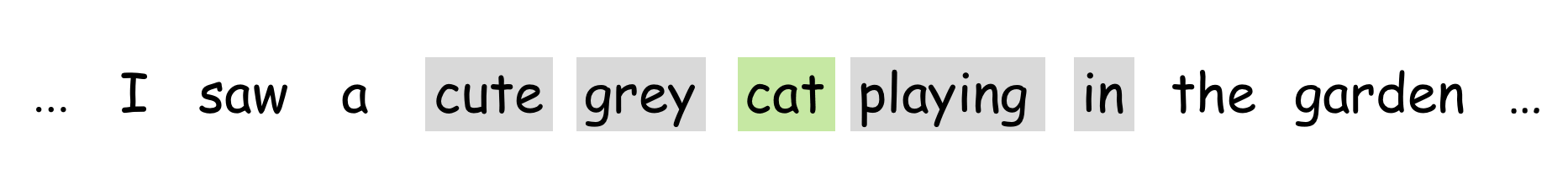
with the central word cat, and four context words. Since we are going to look at just one step, we will pick only one of the context words; for example, let's take cute. Then the loss term for the central word cat and the context word cute is: \[ J_{t,j}(\theta)= -\log P(\color{#888}{cute}\color{black}|\color{#88bd33}{cat}\color{black}) = -\log \frac{\exp\color{#888}{u_{cute}^T}\color{#88bd33}{v_{cat}}}{ \sum\limits_{w\in Voc}\exp{\color{#888}{u_w^T}\color{#88bd33}{v_{cat}} }} = -\color{#888}{u_{cute}^T}\color{#88bd33}{v_{cat}}\color{black} + \log \sum\limits_{w\in Voc}\exp{\color{#888}{u_w^T}\color{#88bd33}{v_{cat}}}\color{black}{.} \]
Note which parameters are present at this step:
- from vectors for central words, only \(\color{#88bd33}{v_{cat}}\);
- from vectors for context words, all \(\color{#888}{u_w}\) (for all words in the vocabulary).
Only these parameters will be updated at the current step.
Below is the schematic illustration of the derivations for this step.
By making an update to minimize \(J_{t,j}(\theta)\), we force the parameters to increase similarity (dot product) of \(\color{#88bd33}{v_{cat}}\) and \(\color{#888}{u_{cute}}\) and, at the same time, to decrease similarity between \(\color{#88bd33}{v_{cat}}\) and \(\color{#888}{u_{w}}\) for all other words \(w\) in the vocabulary.
This may sound a bit strange: why do we want to decrease similarity between \(\color{#88bd33}{v_{cat}}\)
and all other words, if some of them are also valid context words (e.g.,
grey,
playing,
in on our example sentence)?
But do not worry: since we make updates for each context word (and for all central words in your text),
on average over all updates
our vectors will learn
the distribution of the possible contexts.
Try to derive the gradients at the final step of the illustration above.
If you get lost, you can look at the paper
Word2Vec Parameter Learning Explained.
Faster Training: Negative Sampling
In the example above, for each pair of a central word and its context word, we had to update all vectors for context words. This is highly inefficient: for each step, the time needed to make an update is proportional to the vocabulary size.
But why do we have to consider all context vectors in the vocabulary at each step? For example, imagine that at the current step we consider context vectors not for all words, but only for the current target (cute) and several randomly chosen words. The figure shows the intuition.
As before, we are increasing similarity between \(\color{#88bd33}{v_{cat}}\) and \(\color{#888}{u_{cute}}\). What is different, is that now we decrease similarity between \(\color{#88bd33}{v_{cat}}\) and context vectors not for all words, but only with a subset of K "negative" examples.
Since we have a large corpus, on average over all updates we will update each vector sufficient number of times, and the vectors will still be able to learn the relationships between words quite well.
Formally, the new loss function for this step is: \[ J_{t,j}(\theta)= -\log\sigma(\color{#888}{u_{cute}^T}\color{#88bd33}{v_{cat}}\color{black}) - \sum\limits_{w\in \{w_{i_1},\dots, w_{i_K}\}}\log\sigma({-\color{#888}{u_w^T}\color{#88bd33}{v_{cat}}}\color{black}), \] where \(w_{i_1},\dots, w_{i_K}\) are the K negative examples chosen at this step and \(\sigma(x)=\frac{1}{1+e^{-x}}\) is the sigmoid function.
Note that \(\sigma(-x)=\frac{1}{1+e^{x}}=\frac{1\cdot e^{-x}}{(1+e^{x})\cdot e^{-x}} = \frac{e^{-x}}{1+e^{-x}}= 1- \frac{1}{1+e^{x}}=1-\sigma(x)\). Then the loss can also be written as: \[ J_{t,j}(\theta)= -\log\sigma(\color{#888}{u_{cute}^T}\color{#88bd33}{v_{cat}}\color{black}) - \sum\limits_{w\in \{w_{i_1},\dots, w_{i_K}\}}\log(1-\sigma({\color{#888}{u_w^T}\color{#88bd33}{v_{cat}}}\color{black})). \]
How the gradients and updates change when using negative sampling?
The Choice of Negative Examples
Each word has only a few "true" contexts. Therefore, randomly chosen words are very likely to be "negative", i.e. not true contexts. This simple idea is used not only to train Word2Vec efficiently but also in many other applications, some of which we will see later in the course.
Word2Vec randomly samples negative examples based on the empirical distribution of words. Let \(U(w)\) be a unigram distribution of words, i.e. \(U(w)\) is the frequency of the word \(w\) in the text corpus. Word2Vec modifies this distribution to sample less frequent words more often: it samples proportionally to \(U^{3/4}(w)\).
Word2Vec variants: Skip-Gram and CBOW
There are two Word2Vec variants: Skip-Gram and CBOW.
Skip-Gram is the model we considered so far: it predicts context words given the central word. Skip-Gram with negative sampling is the most popular approach.
CBOW (Continuous Bag-of-Words) predicts the central word from the sum of context vectors. This simple sum of word vectors is called "bag of words", which gives the name for the model.
How the loss function and the gradients change for the CBOW model?
If you get lost, you can again look at the paper
Word2Vec Parameter Learning Explained.
Additional Notes
The original Word2Vec papers are:
- Efficient Estimation of Word Representations in Vector Space
- Distributed Representations of Words and Phrases and their Compositionality
You can look into them for the details on the experiments, implementation and hyperparameters. Here we will provide some of the most important things you need to know.
The Idea is Not New
The idea to learn word vectors (distributed representations) is not new. For example, there were attempts to learn word vectors as part of a larger network and then extract the embedding layer. (For the details on the previous methods, you can look, for example, at the summary in the original Word2Vec papers).
What was very unexpected in Word2Vec, is its ability to learn high-quality word vectors very fast on huge datasets and for large vocabularies. And of course, all the fun properties we will see in the Analysis and Interpretability section quickly made Word2Vec very famous.
Why Two Vectors?
As you remember, in Word2Vec we train two vectors for each word: one when it is a central word and another when it is a context word. After training, context vectors are thrown away.
This is one of the tricks that made Word2Vec so simple. Look again at the loss function (for one step): \[ J_{t,j}(\theta)= -\color{#888}{u_{cute}^T}\color{#88bd33}{v_{cat}}\color{black} - \log \sum\limits_{w\in V}\exp{\color{#888}{u_w^T}\color{#88bd33}{v_{cat}}}\color{black}{.} \] When central and context words have different vectors, both the first term and dot products inside the exponents are linear with respect to the parameters (the same for the negative training objective). Therefore, the gradients are easy to compute.
Repeat the derivations (loss and the gradients) for the case with one vector for each word (\(\forall w \ in \ V, \color{#88bd33}{v_{w}}\color{black}{ = }\color{#888}{u_{w}}\) ).
While the standard practice is to throw away context vectors, it was shown that averaging word and context vectors may be more beneficial. More details are here.
Better training
There's one more trick: learn more from this exercise in the Research Thinking section.
Relation to PMI Matrix Factorization
Word2Vec SGNS (Skip-Gram with Negative Sampling) implicitly approximates the factorization of a (shifted) PMI matrix. Learn more here.
The Effect of Window Size
The size of the sliding window has a strong effect on the resulting vector similarities. For example, this paper notes that larger windows tend to produce more topical similarities (i.e. dog, bark and leash will be grouped together, as well as walked, run and walking), while smaller windows tend to produce more functional and syntactic similarities (i.e. Poodle, Pitbull, Rottweiler, or walking, running, approaching).
(Somewhat) Standard Hyperparameters
As always, the choice of hyperparameters usually depends on the task at hand; you can look at the original papers for more details.Somewhat standard setting is:
- Model: Skip-Gram with negative sampling;
- Number of negative examples: for smaller datasets, 15-20; for huge datasets (which are usually used) it can be 2-5.
- Embedding dimensionality: frequently used value is 300, but other variants (e.g., 100 or 50) are also possible. For theoretical explanation of the optimal dimensionality, take a look at the Related Papers section.
- Sliding window (context) size: 5-10.
GloVe: Global Vectors for Word Representation
The GloVe model is a combination of count-based methods and prediction methods (e.g., Word2Vec). Model name, GloVe, stands for "Global Vectors", which reflects its idea: the method uses global information from corpus to learn vectors.
As we saw earlier, the simplest count-based method uses co-occurrence counts to measure the association between word w and context c: N(w, c). GloVe also uses these counts to construct the loss function:
Similar to Word2Vec, we also have different vectors for central and context words - these are our parameters. Additionally, the method has a scalar bias term for each word vector.
What is especially interesting, is the way GloVe controls the influence of rare and frequent words: loss for each pair (w, c) is weighted in a way that
- rare events are penalized,
- very frequent events are not over-weighted.
Lena: The loss function looks reasonable as it is, but the original GloVe paper has very nice motivation leading to the above formula. I will not provide it here (I have to finish the lecture at some point, right?..), but you can read it yourself - it's really, really nice!
Evaluation of Word Embeddings
How can we understand that one method for getting word embeddings is better than another? There are two types of evaluation (not only for word embeddings): intrinsic and extrinsic.
Intrinsic Evaluation: Based on Internal Properties
This type of evaluation looks at the internal properties of embeddings, i.e. how well they capture meaning. Specifically, in the Analysis and Interpretability section, we will discuss in detail how we can evaluate embeddings on word similarity and word analogy tasks.
Extrinsic Evaluation: On a Real Task
This type of evaluation tells which embeddings are better for the task you really care about (e.g.,
text classification, coreference resolution, etc.).
In this setting, you have to train the model/algorithm for the real task several times: one model for each of the
embeddings you want to evaluate. Then, look at the quality of these models to decide which
embeddings are better.
How to Choose?
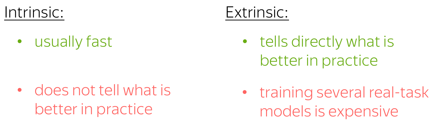
One thing you have to get used to is that there is no perfect solution and no right answer for all situations: it always depends on many things.
Regarding evaluation, you usually care about quality of the task you want to solve. Therefore, you are likely to be more interested in extrinsic evaluation. However, real-task models usually require a lot of time and resources to train, and training several of them may be too expensive.
In the end, this is your call to make :)
Analysis and Interpretability
Lena: For word embeddings, most of the content of this part is usually considered as evaluation (intrinsic evaluation). However, since looking at what a model learned (beyond task-specific metrics) is the kind of thing people usually do for analysis, I believe it can be presented here, in the analysis section.
Take a Walk Through Space... Semantic Space!
Semantic spaces aim to create representations of natural language that capture meaning. We can say that (good) word embeddings form semantic space and will refer to a set of word vectors in a multi-dimensional space as "semantic space".
Below is shown semantic space formed by GloVe vectors trained on twitter data (taken from gensim). Vectors were projected to two-dimensional space using t-SNE; these are only the top-3k most frequent words.
How to: Walk through semantic space and try to find:
- language clusters: Spanish, Arabic, Russian, English. Can you find more languages?
- clusters for: food, family, names, geographical locations. What else can you find?
Nearest Neighbors
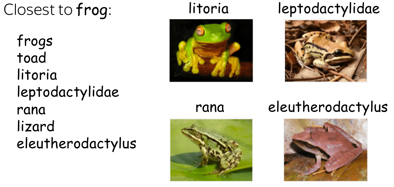
The example is
from the GloVe project page.
During your walk through semantic space, you probably noticed that the points (vectors) which are nearby usually have close meaning. Sometimes, even rare words are understood very well. Look at the example: the model understood that words such as leptodactylidae or litoria are close to frog.
Several pairs from the
Rare Words similarity benchmark.
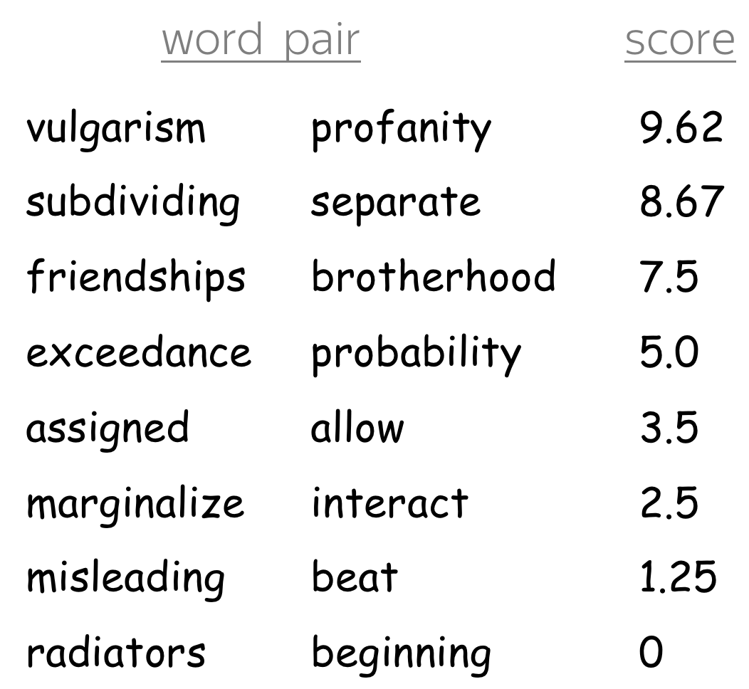
Word Similarity Benchmarks
"Looking" at nearest neighbors (by cosine similarity or Euclidean distance) is one of the methods to estimate the quality of the learned embeddings. There are several word similarity benchmarks (test sets). They consist of word pairs with a similarity score according to human judgments. The quality of embeddings is estimated as the correlation between the two similarity scores (from model and from humans).
Linear Structure
While similarity results are encouraging, they are not surprising: all in all, the embeddings were trained specifically to reflect word similarity. What is surprising, is that many semantic and syntactic relationships between words are (almost) linear in word vector space.
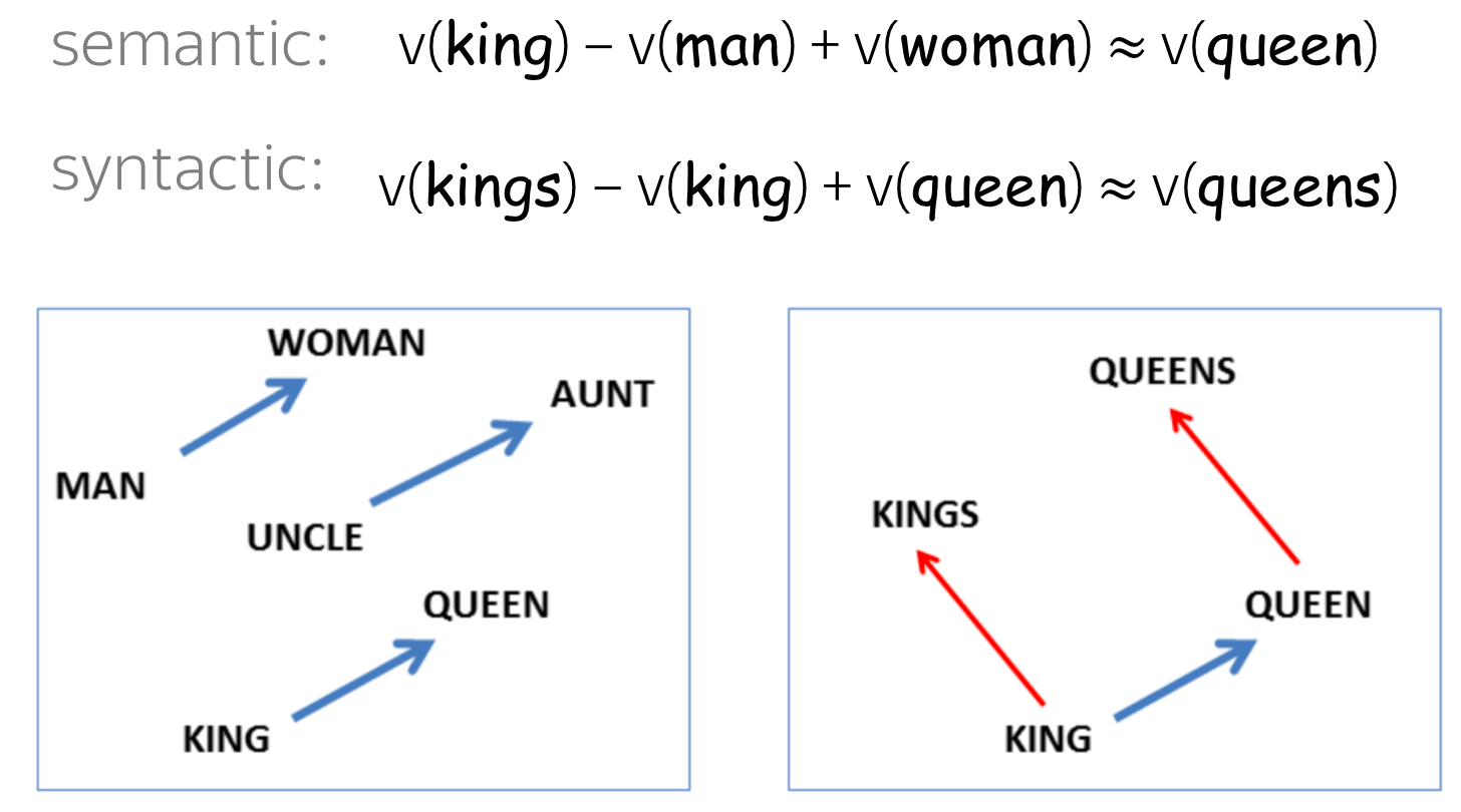
For example, the difference between king and queen is (almost) the same as between man and woman. Or a word that is similar to queen in the same sense that kings is similar to king turns out to be queens. The man-woman \(\approx\) king-queen example is probably the most popular one, but there are also many other relations and funny examples.
Below are examples for the country-capital relation and a couple of syntactic relations.
At ICML 2019, it was shown that there's actually a theoretical explanation for
analogies in Word2Vec.
More details are here.
Lena: This paper,
Analogies Explained: Towards Understanding Word Embeddings
by Carl Allen and Timothy Hospedales from the University of Edinburgh, received
Best Paper Honourable Mention award at ICML 2019 - well deserved!
Word Analogy Benchmarks
These near-linear relationships inspired a new type of evaluation: word analogy evaluation.
Examples of relations and word pairs from
the Google analogy test set.
Given two word pairs for the same relation, for example (man, woman) and (king, queen), the task is to check if we can identify one of the words based on the rest of them. Specifically, we have to check if the closest vector to king - man + woman corresponds to the word queen.
Now there are several analogy benchmarks; these include the standard benchmarks (MSR + Google analogy test sets) and BATS (the Bigger Analogy Test Set).
Similarities across Languages
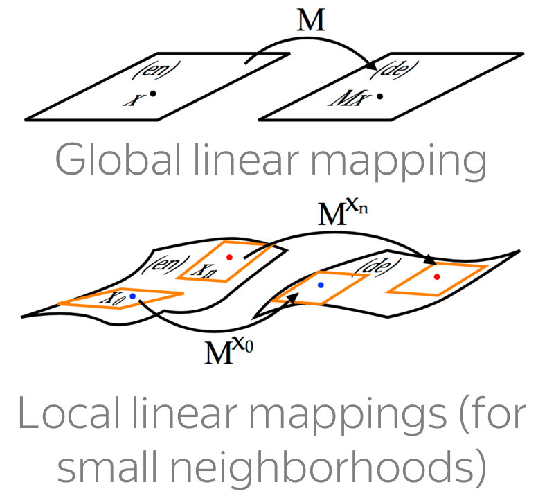
We just saw that some relationships between words are (almost) linear in the embedding space. But what happens across languages? Turns out, relationships between semantic spaces are also (somewhat) linear: you can linearly map one semantic space to another so that corresponding words in the two languages match in the new, joint semantic space.
The figure above illustrates the approach proposed by Tomas Mikolov et al. in 2013 not long after the original Word2Vec. Formally, we are given a set of word pairs and their vector representations \(\{\color{#88a635}{x_i}\color{black}, \color{#547dbf}{z_i}\color{black} \}_{i=1}^n\), where \(\color{#88a635}{x_i}\) and \(\color{#547dbf}{z_i}\) are vectors for i-th word in the source language and its translation in the target. We want to find a transformation matrix W such that \(W\color{#547dbf}{z_i}\) approximates \(\color{#88a635}{x_i}\) : "matches" words from the dictionary. We pick \(W\) such that \[W = \arg \min\limits_{W}\sum\limits_{i=1}^n\parallel W\color{#547dbf}{z_i}\color{black} - \color{#88a635}{x_i}\color{black}\parallel^2,\] and learn this matrix by gradient descent.
In the original paper, the initial vocabulary consists of the 5k most frequent words with their translations, and the rest is learned.
Later it turned out, that we don't need a dictionary at all - we can build a mapping between semantic spaces even if we know nothing about languages! More details are here.
Is the "true" mapping between languages indeed linear, or more complicated? We can look at geometry of the learned semantic spaces and check. More details are here.
The idea to linearly map different embedding sets to (nearly) match them can also be used for a very different task! Learn more in the Research Thinking section.
Research Thinking
Count-Based Methods
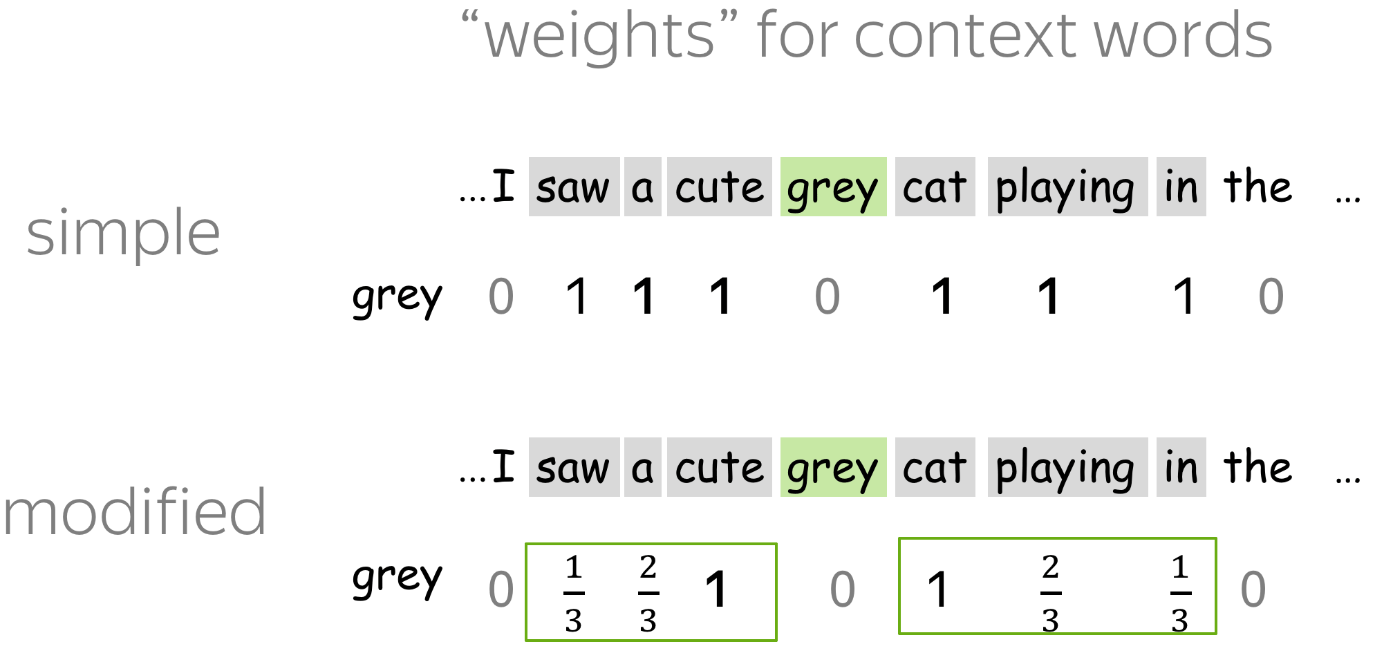
The simplest co-occurrence counts treat context words equally, although these words are at different relative positions from the central word. For example, from one sentence the central word cat will get a co-occurrence count of 1 for each of the words cute, grey, playing, in (look at the example to the right).
Possible answers
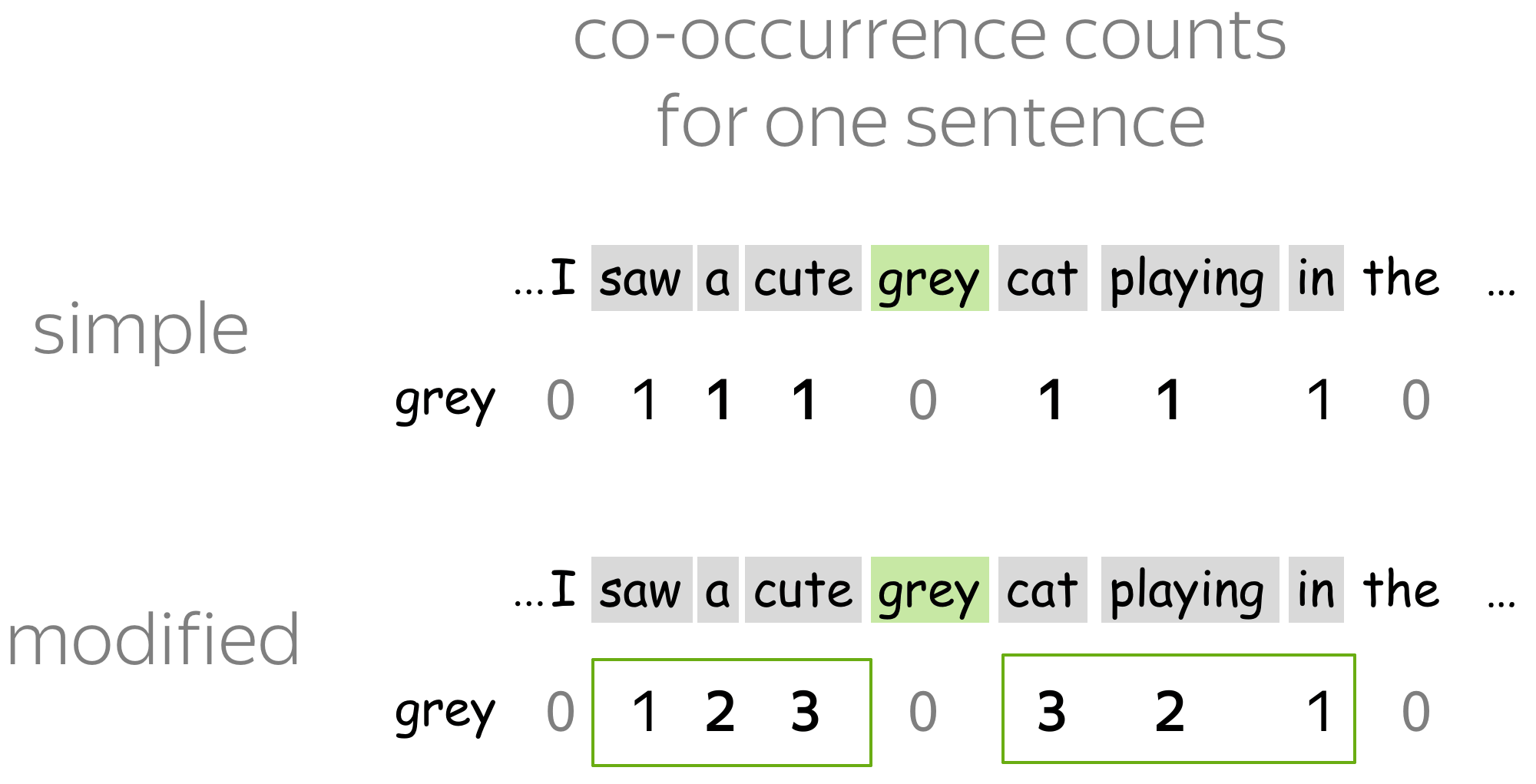 Intuitively, words that are closer to the central are more important; for example,
immediate neighbors are more informative than words at distance 3.
Intuitively, words that are closer to the central are more important; for example,
immediate neighbors are more informative than words at distance 3.
We can use this to modify the model: when evaluating counts, let's give closer words more weight. This idea was used in the HAL model (1996), which once was very famous. They modified counts as shown in the example.
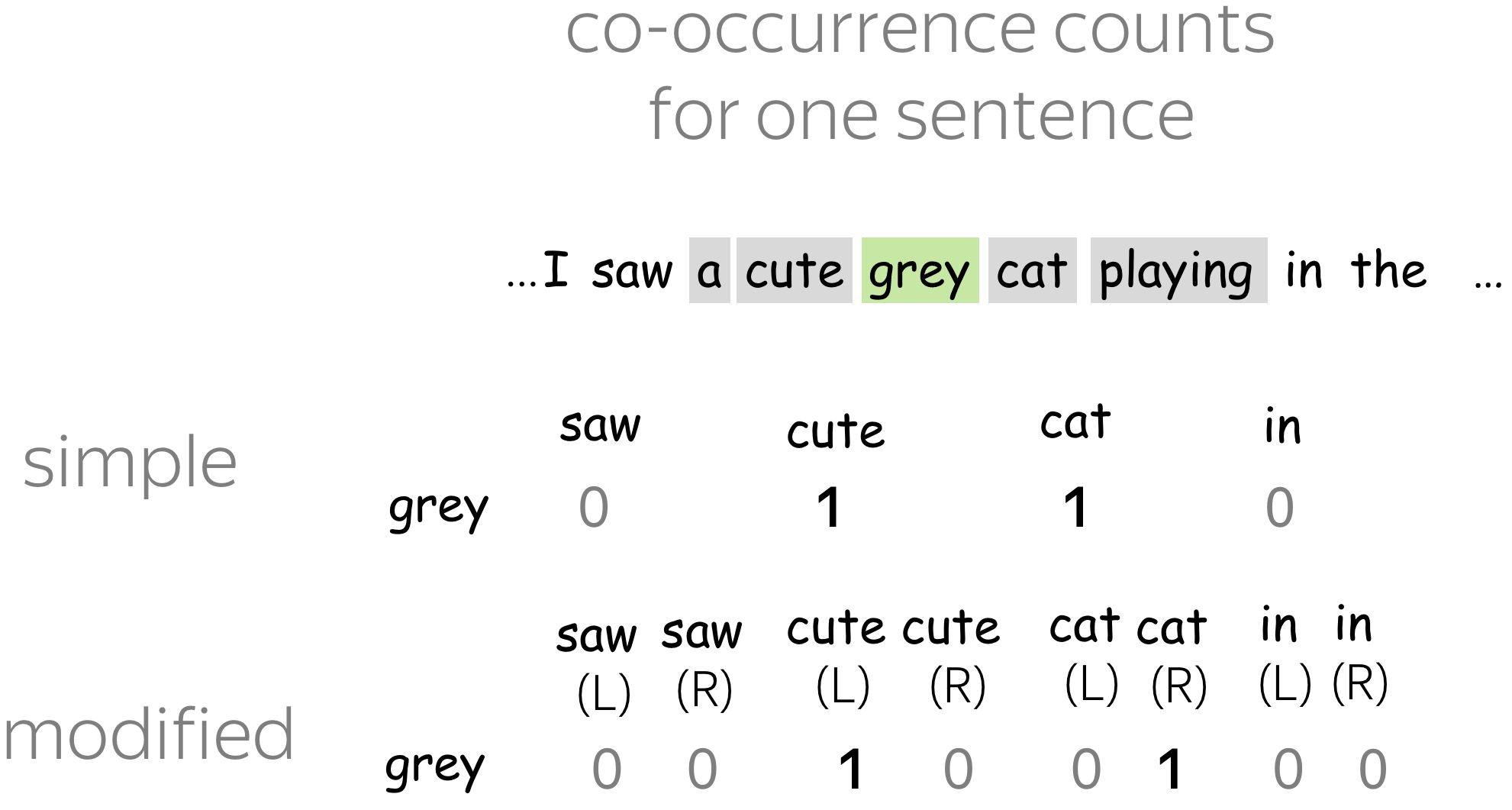
? In language, word order is important; specifically, left and right contexts have different meanings. How can we distinguish between the left and right contexts?
One of the existing approaches
 Here the weighting idea we saw above would not work: we can not say which
contexts, left or right, are more important.
Here the weighting idea we saw above would not work: we can not say which
contexts, left or right, are more important.What we have to do is to evaluate co-occurrences to the left and to the right separately. For each context word, we will have two different counts: one when it is a left context and another when it is the right context. This means that our co-occurrence matrix will have |V| rows and 2|V| columns. This idea was also used in the HAL model (1996).
Look at the example; note that for cute, we have left co-occurrence count, for cat - right.
Word2Vec
During Word2Vec training, we make an update for each of the context words. For example, for the central word cat we make an update for each of the words cute, grey, playing, in.
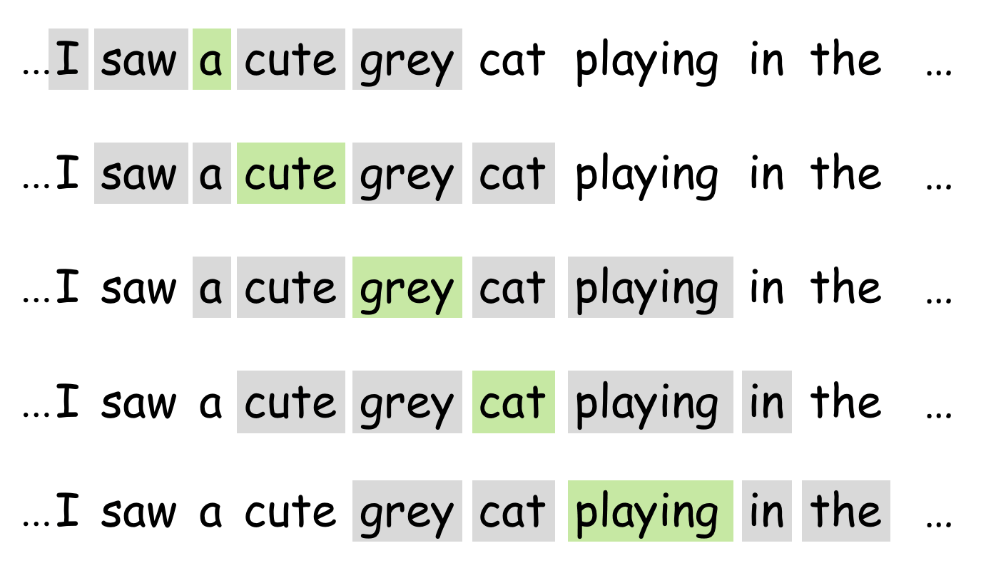
Which word types give more/less information than others? Think about some characteristics of words that can influence their importance. Do not forget the previous exercise!
Possible answers
- word frequency
We can expect that frequent words usually give less information than rare ones. For example, the fact that cat appears in context of in does not tell us much about the meaning of cat: the word in serves as a context for many other words. In contrast, cute, grey and playing already give us some idea about cat. -
distance from the central word
As we discussed in the previous exercise on count-based methods, words that are closer to the central may be more important.
? How can we use this to modify training?
Tricks from the original Word2Vec
1. Word Frequency

Interestingly, this heuristic works well in practice: it accelerates learning and even significantly improves the accuracy of the learned vectors of the rare words.
2. Distance from the central word
 As in the previous exercise
on count-based methods, we can assign higher weights to the words which are closer to
the central.
As in the previous exercise
on count-based methods, we can assign higher weights to the words which are closer to
the central.
At the first glance, you won't see any weights in the original Word2Vec implementation. However, at each step it samples the size of the context window from 1 to L. Therefore, words which are closer to central are used more frequently than the distant ones. In the original work this was (probably) done for efficiency (fewer updates for each step), but this also has the effect similar to assigning weights.
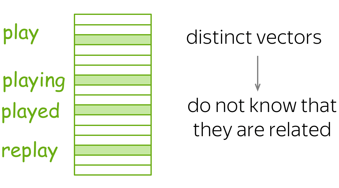
Usually, we have a look-up table where each word is assigned a distinct vector. By construction, these vectors do not have any idea about subwords they consist of: all information they have is what they learned from contexts.
Possible answers
- better understanding of morphology
By assigning a distinct vector to each word, we ignore morphology. Giving information about subwords can let the model know that different tokens can be forms of the same word. - representations for unknown words
Usually, we can represent only those words, which are present in the vocabulary. Giving information about subwords can help to represent out-of-vocabulary words relying of their spelling. - handling misspellings
Even if one character in a word is wrong, this is another token, and, therefore, a completely different embedding (or even unknown word). With information about subwords, misspelled word would still be similar to the original one.
? How can we incorporate information about subwords into embeddings? Let's assume that the training pipeline is fixed, e.g., Skip-Gram with Negative sampling.
One of the existing approaches (FastText)
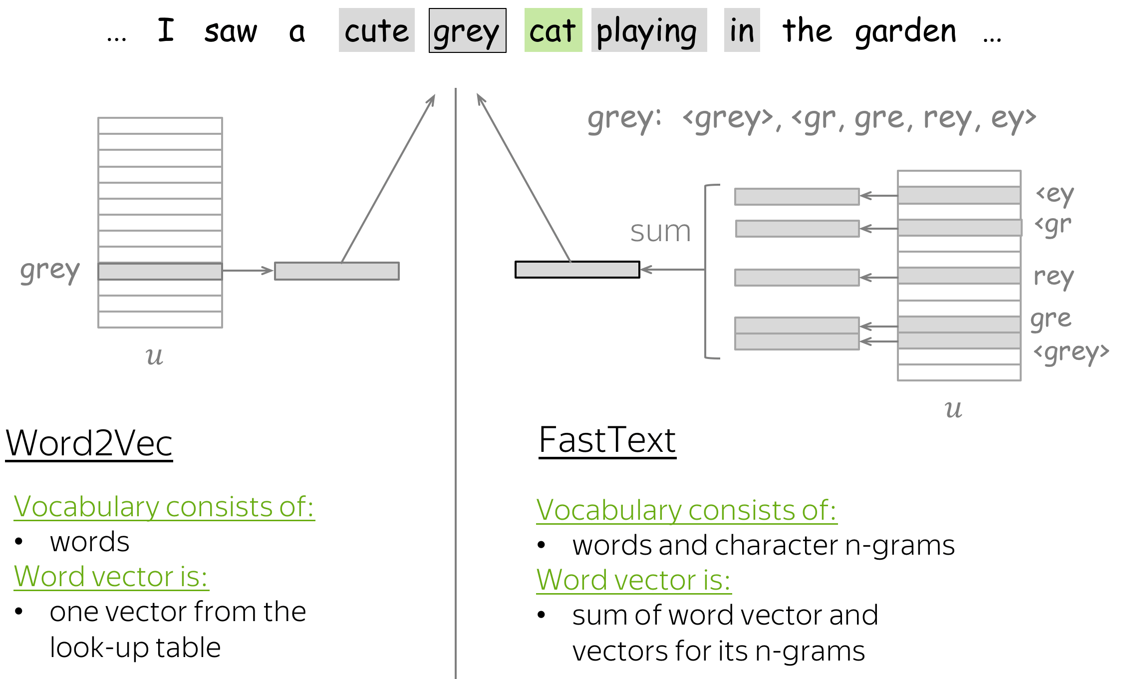
Note that this changes only the way we form word vector; the whole training pipeline is the same as in the standard Word2Vec.
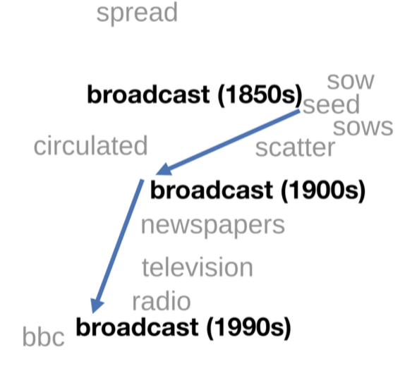
Semantic Change
Imagine you have text corpora from different sources: time periods, populations, geographic regions, etc. In digital humanities and computational social science, people often want to find words that used differently in these corpora.
Some of the existing attempts
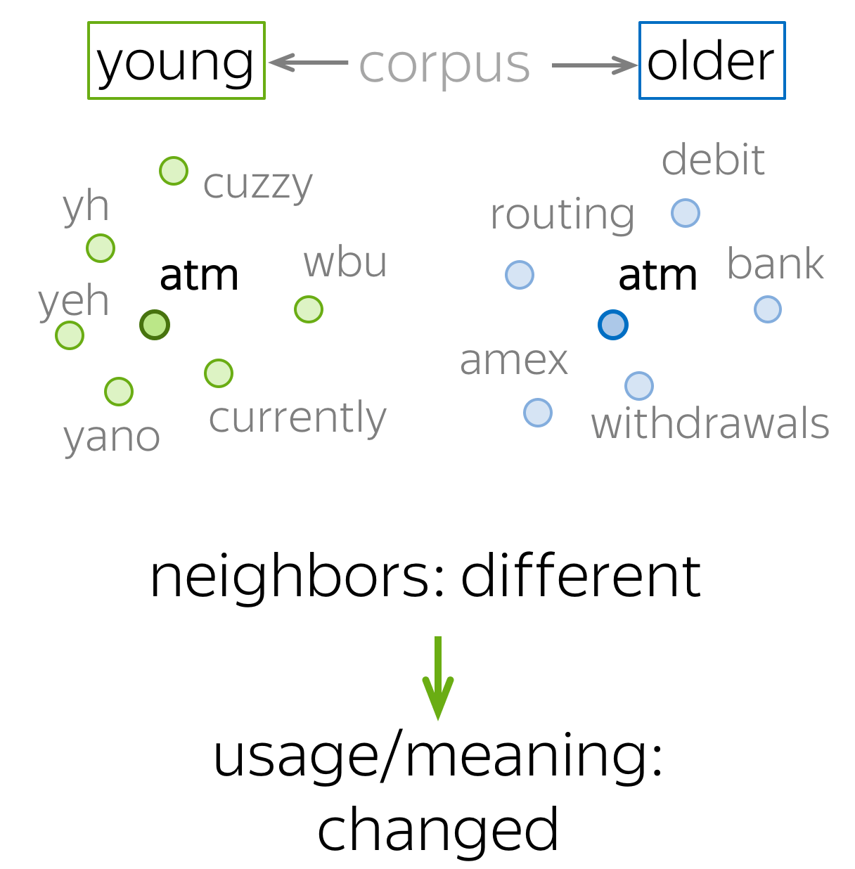
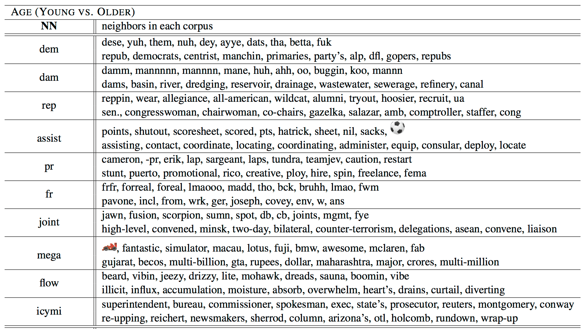
ACL 2020: train embeddings, look at the neighbors
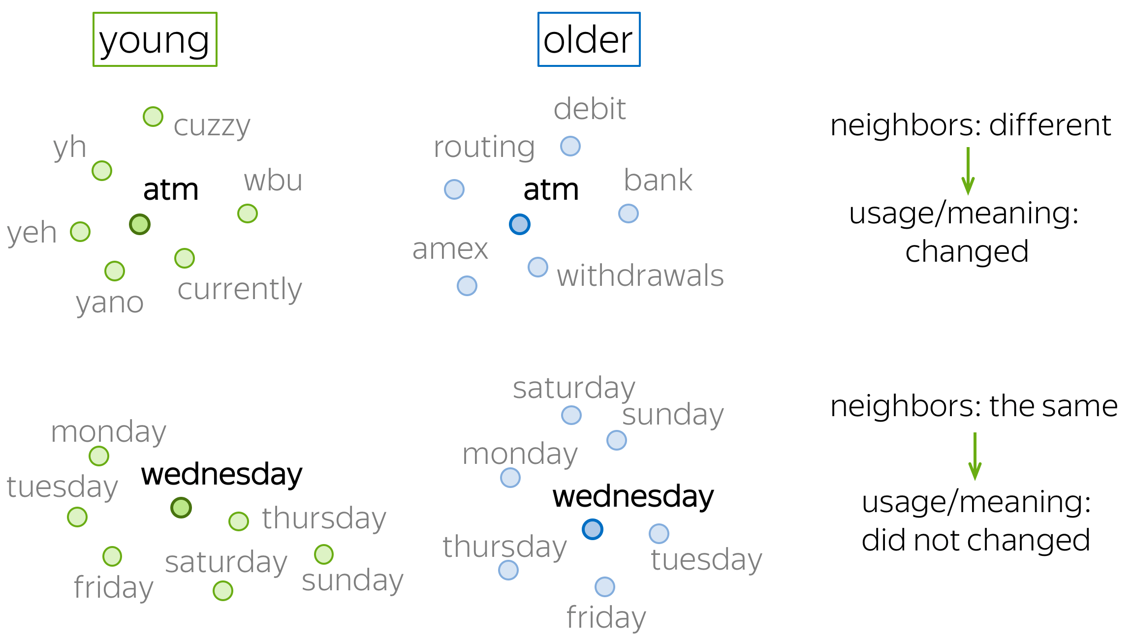 A very simple approach
is to train embeddings (e.g., Word2Vec) and look at the closest neighbors.
If a word's closest neighbors are different for the two corpora, the word changed
its meaning: remember that word embeddings reflect contexts they saw!
A very simple approach
is to train embeddings (e.g., Word2Vec) and look at the closest neighbors.
If a word's closest neighbors are different for the two corpora, the word changed
its meaning: remember that word embeddings reflect contexts they saw!
This approach was proposed in this ACL 2020 paper. Formally, for each word the authors take k nearest neighbors in the two embeddings sets and count how many neighbors are the same. Large intersection means that the meaning is not different, small intersection - meaning is different.
Lena: Note that while the approach is recent, it is extremely simple and works better than previous more complicated ideas. Never be afraid to try simple things - you'll be surprised how often they work!
Previous popular approach: align two embedding sets
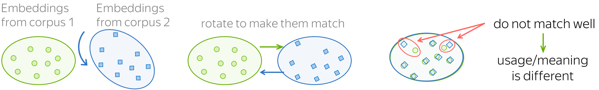
Lena: You will implement Ortogonal Proctustes in your homework to align Russian and Ukranian embeddings. Find the notebook in the course repo.
Related Papers
What's inside:
- Good Old Classics
- Analyzing Geometry
- Biases in Word Embeddings
- Semantic Change
- Theory to the Rescue! - coming soon
- Cross-Lingual Embeddings - coming soon
- ... to be updated
Good Old Classics
Theoretically, Word2Vec is not so different from matrix factorization approaches! Skip-gram with negative-sampling (SGNS) implicitly factorizes the shifted pointwise mutual information (PMI) matrix: \(PMI(\color{#88bd33}{w}\color{black}, \color{#888}{c}\color{black})-\log k\), where \(k\) is the number of negative examples in negative sampling.
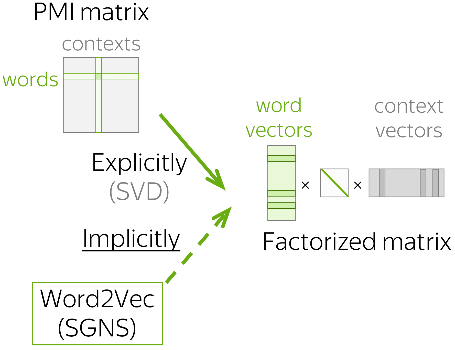
More details
Let us recall the loss function for central word w and context word c: \[ J_{\color{#88bd33}{w}\color{black}, \color{#888}{c}}\color{black}(\theta)= \log\sigma(\color{#888}{u_{c}^T}\color{#88bd33}{v_{w}}\color{black}) + \sum\limits_{\color{#888}{ctx}\color{black}\in \{w_{i_1},\dots, w_{i_k}\}} \log(1-\sigma({\color{#888}{u_{ctx}^T}\color{#88bd33}{v_w}}\color{black})), \] where \(w_{i_1},\dots, w_{i_K}\) are the \(k\) negative examples chosen at this step.This is the loss for one step, but how the loss for the whole corpus will look like? Surely we will meet the same word-context pairs several times.
We will meet:
- (w, c) word-context pair: \(N(\color{#88bd33}{w}\color{black}, \color{#888}{c}\color{black})\) times;
- c as negative example for
w:
\( \frac{kN(\color{#88bd33}{w}\color{black})N(\color{#888}{c}\color{black})}{N}\) times.
Why: each time we sample a negative example, we can pick c with the probability \(\frac{N(\color{#888}{c}\color{black})}{N}\) - frequency of c. Multiply by N(w) because we meet w exactly N(w) times; multiply by \(k\) because we sample \(k\) negative examples.
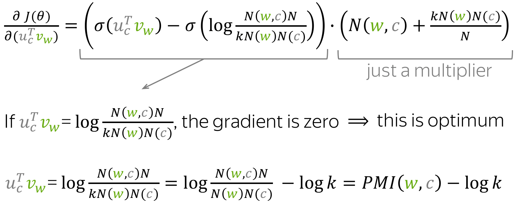
This is a rather intuitive explanation of the idea behind the proof. For more formal version, look in the paper. Additionally, the authors use these results to factorize the shifted PMI matrix directly and to see if the quality is the same as Word2Vec.
At some point, it was believed that prediction-based embeddings are better than count-based. But this is not true: we can adapt some "tricks" from the word2vec implementation to count-based models and achieve the same results. Also, when evaluated properly, GloVE is worse than Word2Vec.
More details
The paper tests many hyperparameters and has lots of experiments - I do recommend looking into it. Here I will provide the most important things you need to remember.
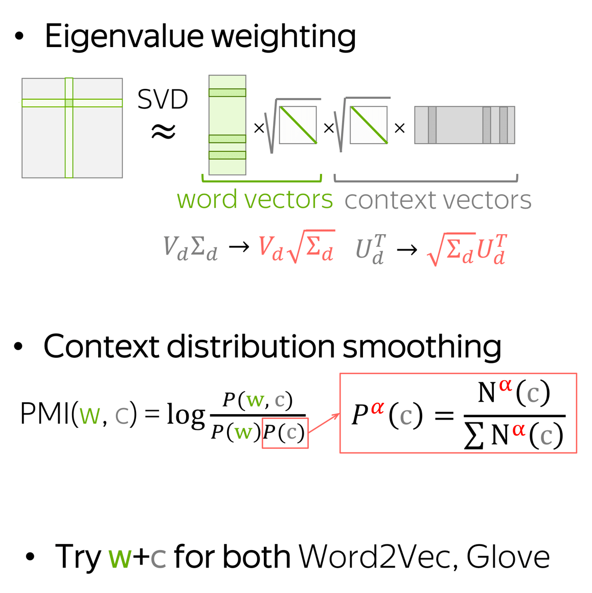
Eigenvalue Weighting: It is better to use SVD "incorrectly"
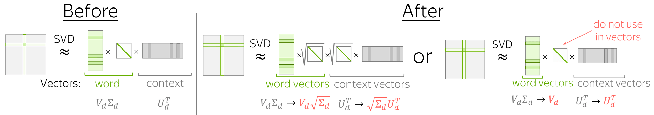
Typically, word and context vectors derived by SVD are represented by \(V_d\Sigma_d\) and \(U_d\): the eigenvalue matrix is included only in word vectors. However, for word similarity tasks this is not the optimal construction. The experiments show that symmetric variants are better: either include \(\sqrt{\Sigma_d}\) in both word and context vectors, or discard in both (look at the figure).
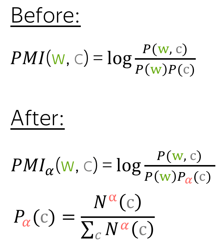
Context Distribution Smoothing
As we discussed in the lecture, Word2Vec samples negative examples according to smoothed unigram distribution \(U^{3/4}\). This was done to pick rare words more frequently.
We can do something similar when calculating PMI: instead of true context distribution, let's use the smoothed one (look at the figure to the right). As in Word2Vec, \(\alpha=0.75\).
Word and Context Vectors in Word2Vec: Try to Average
Recall that after training GloVe averages word and context vectors, while Word2Vec throws context vectors away. However, sometimes Word2Vec can also benefit from averaging: you have to try!
Main Results
- with tuned hyperparameters, prediction-based embeddings are not better than count-based;
- with a couple of fixes, Word2Vec (SGNS) is better than GloVe on every task.
Analyzing Geometry
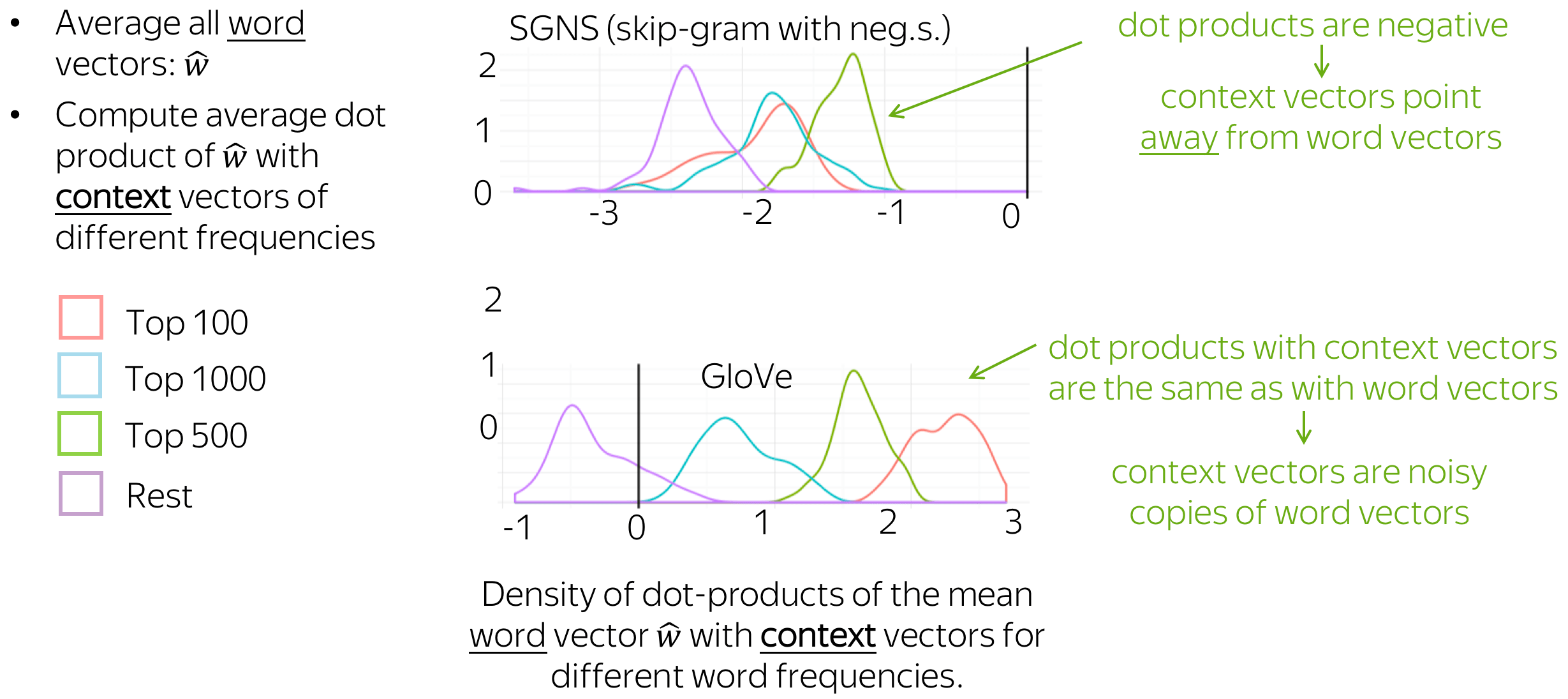
The negative sampling objective influences the geometry of embeddings: word vectors \(\color{#88bd33}{v_{w}}\) lie in a narrow cone, diametrically opposed to the context vectors \(\color{#888}{u_{w}}\). Also, differently from GloVe, context vectors in Word2Vec point away from word vectors.
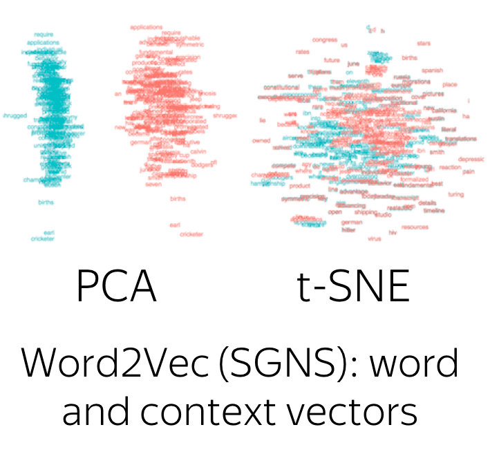
More details
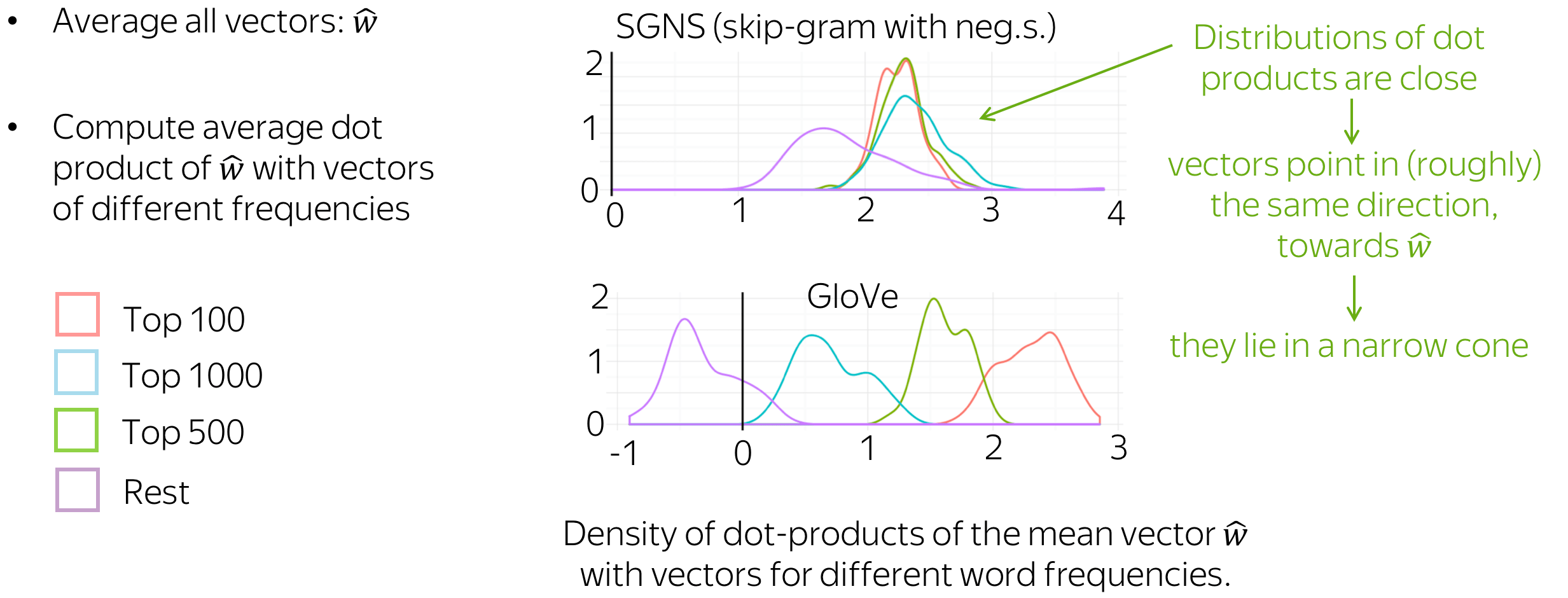
Word vectors point to roughly the same direction
The authors evaluate dot products of vectors for words of different frequencies with the mean of all vectors. Since the distributions are very close and dot products are positive, the vectors (mostly) point in the direction of the mean vector.
Context vectors point away from word vectors
Here we do the same, but take context vectors (the mean is still for word vectors). For SGNS, dot products of context vectors with the mean of word vectors are negative. This means that context vectors point away from word vectors, and it is not reasonable to use them - we throw them away and use only word vectors. For GloVe, this is not the case: context vectors behave the same way as word vectors.
We learned that we can (almost) match semantic spaces for different languages linearly. But is the "true" underlying mapping between languages indeed linear? If it is linear globally, then all local linear mappings have to be similar (to the global linear mapping, and hence to each other). Well, they are not.
More details
How to check if the "true" mapping between semantic spaces is indeed linear? The main idea is shown at the figure.
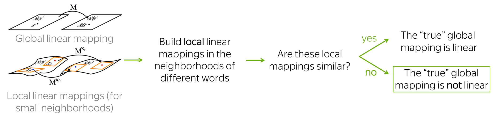
Local cross-lingual mappings are not similar
To check if the local mappings are similar, the authors
- for several words, take their neighborhood: a set of words with the cosine similarity at least some value;
- for each neighborhood, find the corresponding set of words in the other language;
- build local cross-linear mappings;
- evaluate how similar these mappings are: for two mappings \(M_1\) and \(M_2\) (e.g., for neighborhoods of words \(w_1\) and \(w_2\)), compute the cosine similarity between the vectorized versions of matrices \(M_1\) and \(M_2\).
For distant words, their local cross-lingual mappings are different
The authors found that
- local mappings for different neighborhoods can be very different. Therefore, "true" cross-lingual mapping between semantic spaces is not linear;
- for more distant words, the local cross-lingual mappings are more different.
Lena: This is an example of how analysis can improve quality!
The authors noticed that (i) embeddings have non-zero mean and (ii) early singular values are much larger than the rest. When the authors eliminated these properties, they got large improvements in both intrinsic and extrinsic evaluation.
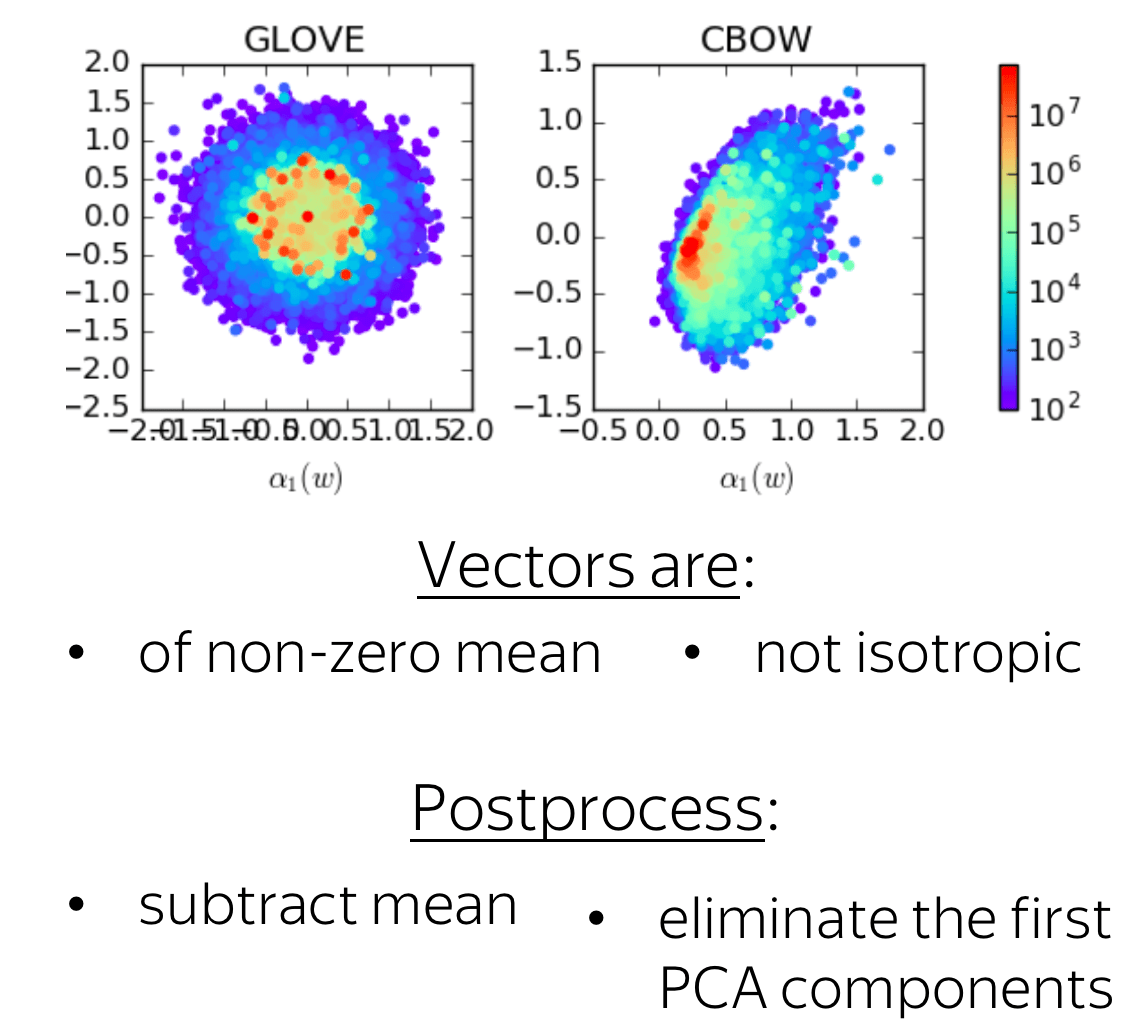
More details
Step 1: Analyze
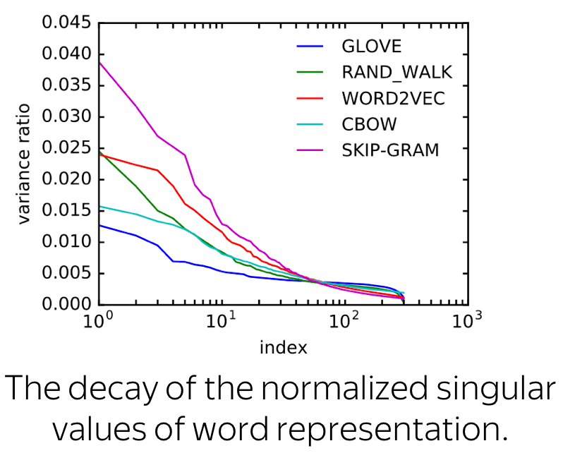
For different word embedding models and languages, the authors found that vectors
- have a large non-zero mean
- are not isotropic
Look at the figure: if \(\sigma_i\) are singular values, then they decay almost exponentially for small \(i\), and remain roughly constant for the rest.
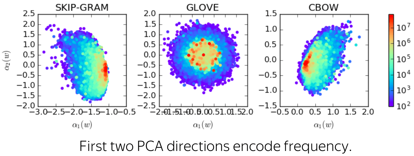
Additionally, the authors noticed that the top PCA components encode something which is not related to semantics: e.g., word frequency.
These properties seem to have nothing to do with semantic, i.e., something which is important for us in word embeddings. What if we eliminate these effects? Will it be better?
Step 2: Use Observations to Improve Quality
To eliminate the found properties, the authors
- subtract from word vectors their mean
- eliminate top PCA components
Let \(u_1, \dots, u_d\) be the PCA components of word vectors \(\{v_w, w\in V\}\). Then the vectors are updated as follows: \[v_w \longleftarrow v_w - \sum\limits_{i=1}^d(u_i^Tv_w)u_i.\]
Result: large improvements in various tasks, both intrinsic (similarity and analogy) and extrinsic (supervised classification).
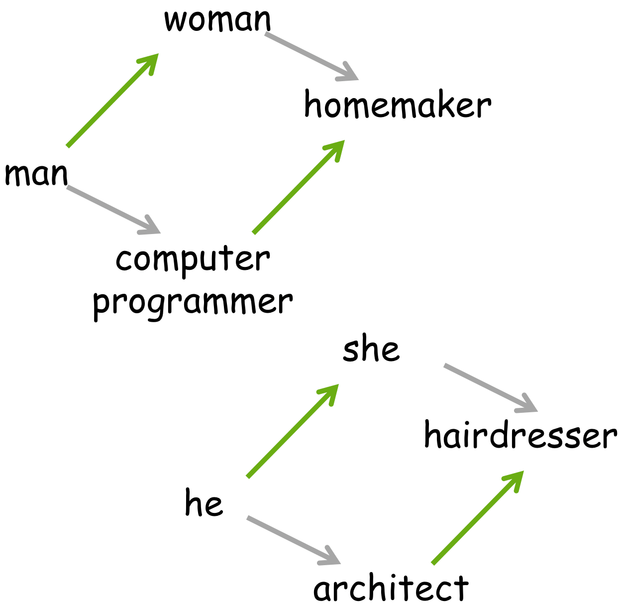
Biases in Word Embeddings
Word embeddings are biased. For example, while their analogical reasoning can be desirable, e.g. "a man to a woman is as a king to a queen", but also "a man to a woman is as a physician to a nurse", which is an undesired association.
More details
Problem: Embeddings are Biased
The authors noticed that word embeddings are biased: they encode undesired gender associations. To find such examples, they take a seed pair (e.g., (a, b) = (he, she)) and find pairs of words which have the same association: differ from each other in the same direction, and relatively close to each other. Formally, they pick pairs with the high score:
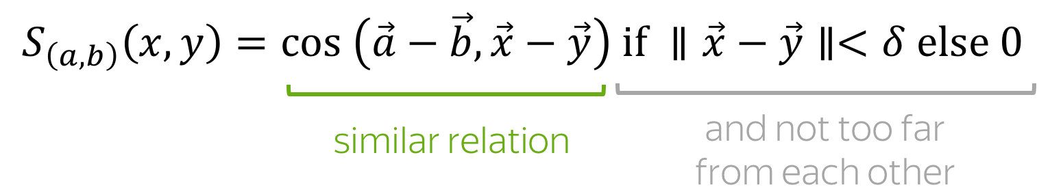
Look at the results below - definitely some pairs are biased!
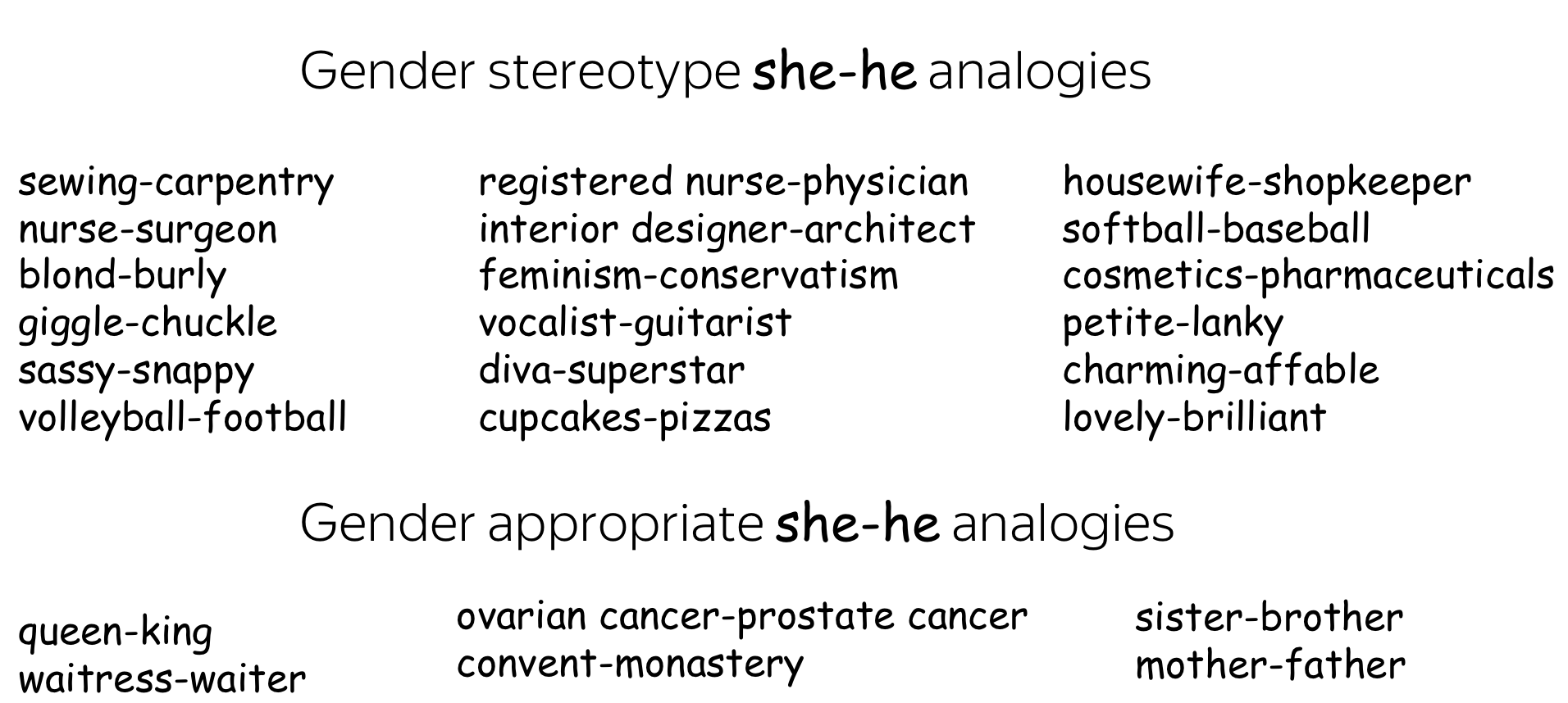
This means that, for example, not only "a man to a woman is as a king to a queen", which is the desired behavior, but also "a man to a woman is as a physician to a nurse", which is an undesired association.
Gender-stereotypic occupations
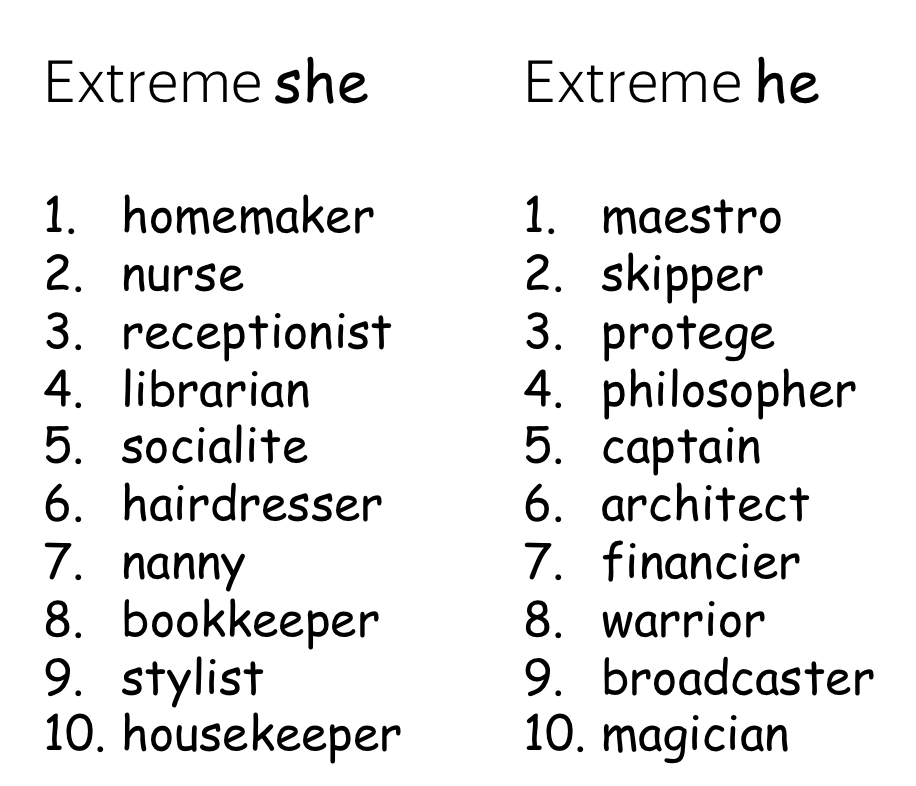
To find the most gender-stereotypic occupations, the authors project occupations onto the he-she gender direction. Results are shown to the right.
We can see that, for example, homemaker, nurse, librarian, stylist are mostly associated with women, while captain, magician, architect, warrior are more strongly associated with men.
Debiasing Word Embeddings
In the original paper, the authors also propose several heuristics to debias word embeddings - remove the undesired associations as a post-processing step. Since a lot has been done on debiasing recently, for more details on this specific approach look in the original paper. For a more recent method, look at the next paper.
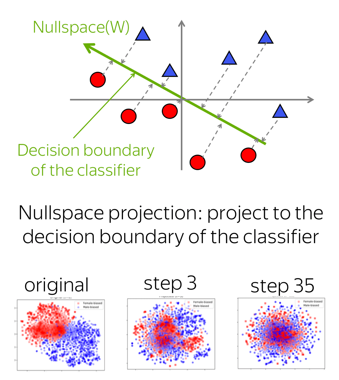
Iterative nullspace projection to debias word embeddings:
- train a linear classifier \(W\) to predict a property from embeddings (e.g., gender),
- linearly project embeddings on the \(W\)'s nullspace (\(x \rightarrow Px\), \(W(Px)=0\)) - remove the information used for prediction;
- repeat until a classifier is not able to predict anything.
More details
Idea: Remove Information Used by a Linear Classifier
We have to remove the information about some desired property (e.g., gender), but not to harm other properties of the embeddings. The authors proposed a very simple idea: train a linear classifier to predict this property from the embeddings, then remove the information this classifier used.
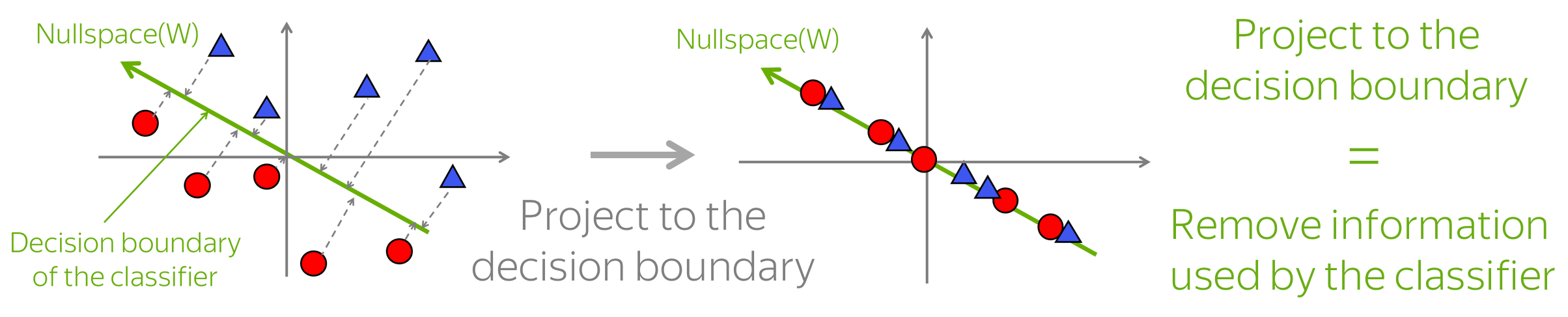
If the classifier is linear, the removing part can be done easily: by projecting onto the classifier's decision boundary. This projection is the least harming way to remove the linear information about the property: it harms the distances between embeddings as little as possible.
The method is iterative: you have to repeat this (train a classifier and project to the new decision boundary) until the classifier is not able to predict anything meaningful. When a classifier can not predict the property, we know that all information has been removed.
Results: All Good
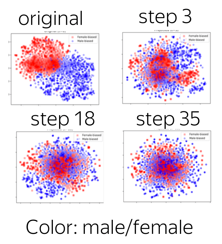
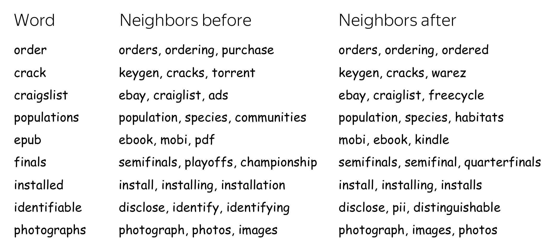
In the original paper, you will find experiments showing that the method:
- does remove bias
(look at the illustration to the right: t-SNE projection of GloVe vectors of the most gender-biased words at 0, 3, 18, 35 iterations of the algorithm), - does not hurt embedding quality
(e.g., look at the closest neighbors before and after debiasing: see below).
For more formal things and more results and examples, look at the original paper.
Semantic Change
Imagine you have text corpora from different sources: time periods, populations, geographic regions, etc. In this part, the task is to find words that used differently in these corpora.
Lena: This paper was used in the Research Thinking section. Here I've hidden from you the links and the content - better go there to think. But if you do want, you can learn about the paper here.
Spoiler alert!

Lena: This paper was used in the Research Thinking section. Here I've hidden from you the links and the content - better go there to think. But if you do want, you can learn about the paper here.
Spoiler alert!
Theory to the Rescue!

Cross-Lingual Embeddings

Have Fun!
next