Information-Theoretic Probing with MDL
 This is a post for the EMNLP 2020 paper
Information-Theoretic Probing with Minimum Description Length.
This is a post for the EMNLP 2020 paper
Information-Theoretic Probing with Minimum Description Length.
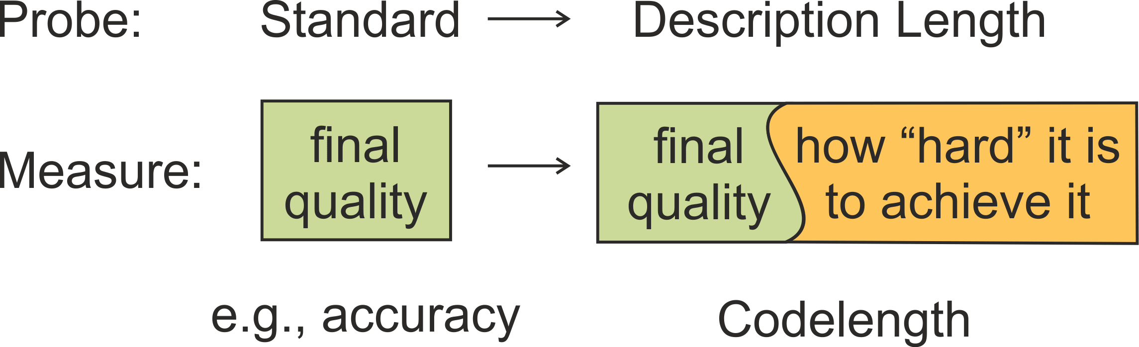
Probing classifiers often fail to adequately reflect differences in representations and can show different results depending on hyperparameters. As an alternative to the standard probes,
- we propose information-theoretic probing which measures minimum description length (MDL) of labels given representations;
- we show that MDL characterizes both probe quality and the amount of effort needed to achieve it;
- we explain how to easily measure MDL on top of standard probe-training pipelines;
- we show that results of MDL probes are more informative and stable than those of standard probes.

 March 2020
How to understand if a model captures a linguistic property?
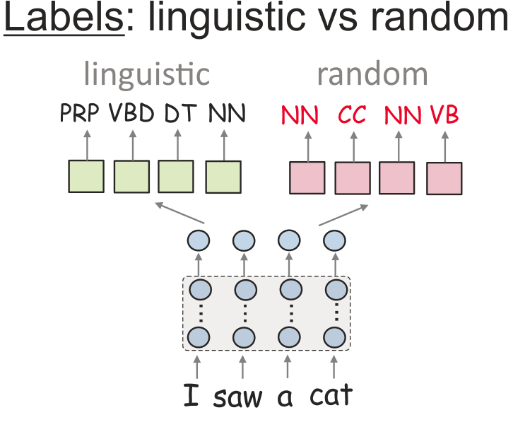
How would you understand whether a model (e.g., ELMO, BERT) learned to encode some linguistic property? Usually this question is narrowed down to the following. We have: dataStandard Probing: train a classifier, use its accuracy
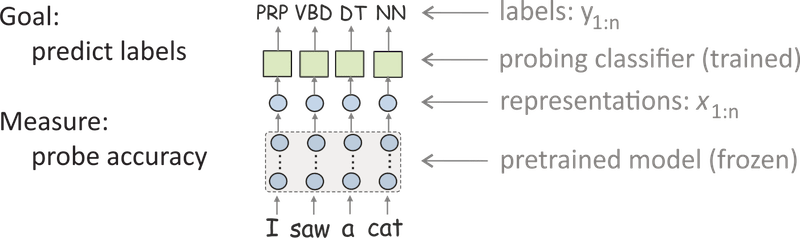 The most popular approach is to use probing classifiers (aka probes, probing tasks, diagnostic classifiers).
These classifiers are trained to predict a linguistic property from frozen representations,
and accuracy of the classifier is used to measure how well these representations encode the property.
Looks reasonable and simple, right? Yes, but...
The most popular approach is to use probing classifiers (aka probes, probing tasks, diagnostic classifiers).
These classifiers are trained to predict a linguistic property from frozen representations,
and accuracy of the classifier is used to measure how well these representations encode the property.
Looks reasonable and simple, right? Yes, but...
Wait, how about some sanity checks?
 While such probes are extremely popular, several 'sanity checks' showed that
differences in accuracies fail to reflect differences in representations.
These sanity checks are different kinds of random baselines. For example,
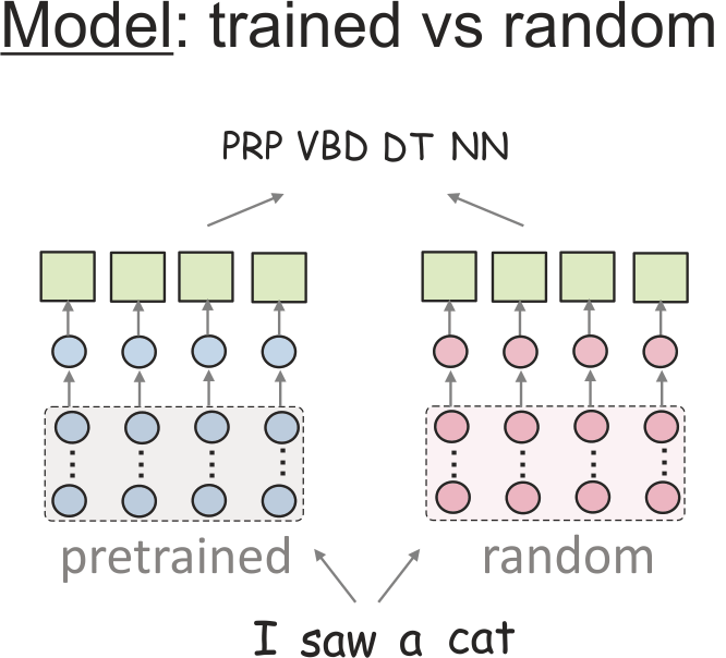
Zhang & Bowman (2018) compared
probe scores for trained models and randomly initialized ones. They were able to see reasonable differences in the scores
only when reducing the amount of a classifier training data.
While such probes are extremely popular, several 'sanity checks' showed that
differences in accuracies fail to reflect differences in representations.
These sanity checks are different kinds of random baselines. For example,
Zhang & Bowman (2018) compared
probe scores for trained models and randomly initialized ones. They were able to see reasonable differences in the scores
only when reducing the amount of a classifier training data.
 Later Hewitt & Liang (2019) proposed to
put probe accuracy in context with its ability to remember from word types. They constructed so-called 'control tasks',
which are manually constructed for each linguistic task. A control task defines random output for a word type,
regardless of context. For example, for POS tags, each word is assigned
a random label based on the empirical distribution of tags.
Control tasks were used to perform an exhaustive search over hyperparameters for training probes and
to find a setting with the largest
difference in the scores. This was achieved by reducing size of a probing model (e.g., fewer neurons).
Later Hewitt & Liang (2019) proposed to
put probe accuracy in context with its ability to remember from word types. They constructed so-called 'control tasks',
which are manually constructed for each linguistic task. A control task defines random output for a word type,
regardless of context. For example, for POS tags, each word is assigned
a random label based on the empirical distribution of tags.
Control tasks were used to perform an exhaustive search over hyperparameters for training probes and
to find a setting with the largest
difference in the scores. This was achieved by reducing size of a probing model (e.g., fewer neurons).
Houston, we have a problem.
We see that accuracy of a probe does not always reflect what we want it to reflect, at least not without explicit search for a setting where it does. But then another problem arises: if we tune a probe to behave in a certain way for one task (e.g., we tune its setting to have low accuracy for a certain control task), how do we know if it's still reasonable for other tasks? Well, we do not (if you do, please tell!). All in all, we want a probing method which does not require a human to tell it what to say.Information-Theoretic Viewpoint
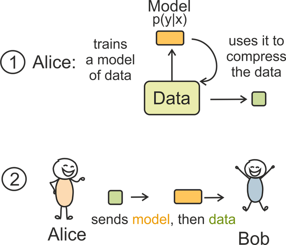
Let us come back to the initial task: we have dataAdventures of Alice, Bob and the Data
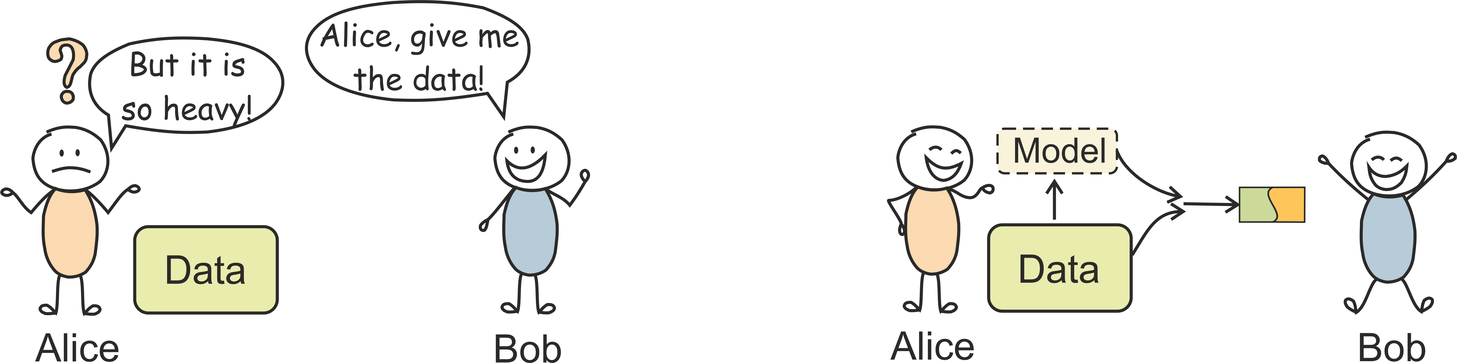 Let us imagine that Alice has all pairs
 Changing a probe's goal converts it into an MDL probe
Turns out that to evaluate MDL we don't need to change much in standard probe-training pipelines. This is done via a simple trick: we know that data can be compressed using some probabilistic modelThe Data Part
TL;DR: cross-entropy is the data codelength
Let's assume for now Alice and Bob have agreed in advance on a model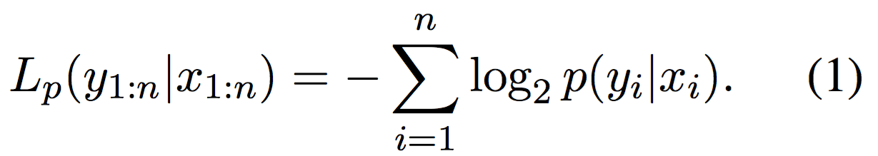
Learning is Compression
Note that (1) is exactly the categorical cross-entropy loss evaluated on the model p. This shows that the task of compressing labelsCompression is compared against Uniform Code
Compression is usually compared against uniform encoding which does not require any learning from data. For K classes, it assumesThe Amount of Effort Part: Strength of the Regularity in the Data
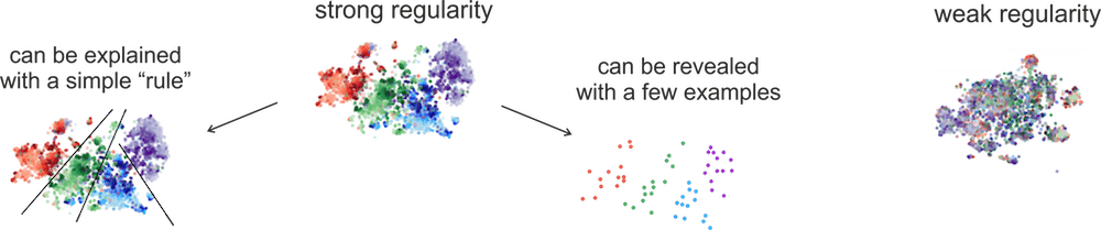 Based on real events! These are t-sne projections of representations of different occurrences of
the token is from the last layer of MT encoder (strong) and the last LM layer (weak).
The colors show CCG tags (only 4 most frequent tags).
Curious why MT and LM behave this way? Look at our
Evolution of Representations post!
Now we come to the other component of the total codelength, which
characterizes how hard it is to achieve final quality of a trained probe. Intuitively,
if representations have some clear structure with respect to labels, this structure can be
understood with
less effort; for example,
Based on real events! These are t-sne projections of representations of different occurrences of
the token is from the last layer of MT encoder (strong) and the last LM layer (weak).
The colors show CCG tags (only 4 most frequent tags).
Curious why MT and LM behave this way? Look at our
Evolution of Representations post!
Now we come to the other component of the total codelength, which
characterizes how hard it is to achieve final quality of a trained probe. Intuitively,
if representations have some clear structure with respect to labels, this structure can be
understood with
less effort; for example,
- the "rule" explaining this structure (i.e., a probing model) can be simple, and/or
- the amount of data needed to reveal this structure can be small.
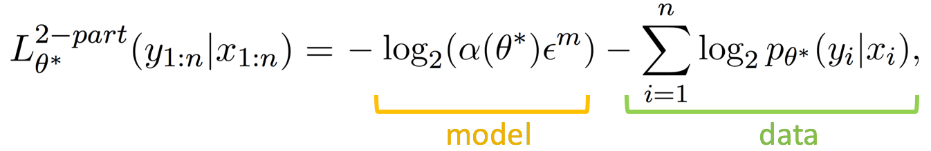
Variational Code: Explicit Transmission of the Model
 Variational code is an instance of two-part codes,
where a model (probe weights) is transmitted explicitly and then used to encode the data.
It has been known for quite a while that
this joint cost (model and data codes) is exactly the loss function of a variational learning methods.
Variational code is an instance of two-part codes,
where a model (probe weights) is transmitted explicitly and then used to encode the data.
It has been known for quite a while that
this joint cost (model and data codes) is exactly the loss function of a variational learning methods.
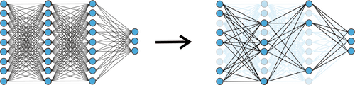
The Idea: Informal version
What is happening in this part:- model weights are transmitted explicitly;
- each weight is treated as a random variable;
- weights with higher variance can be transmitted with lower precision (i.e., fewer bits);
- by choosing sparsity-inducing priors we will obtain induced (sparse) probe architectures.
Codelength: Formal Derivations
I hereby confirm that I'm not afraid of scary formulas

May the force be with you!
Here we assume that Alice and Bob have agreed on a model class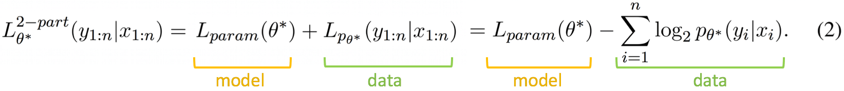

We Use: Bayesian Compression
 You can choose priors for weights to get something interesting. For example, if you choose
sparsity-inducing priors on the parameters, you can get
variational dropout.
What is more interesting, you can do this in such way that you prune the whole neurons (not just individual weights): this is the
Bayesian network compression method we use.
This allows us to assess the probe complexity
both using its description length
You can choose priors for weights to get something interesting. For example, if you choose
sparsity-inducing priors on the parameters, you can get
variational dropout.
What is more interesting, you can do this in such way that you prune the whole neurons (not just individual weights): this is the
Bayesian network compression method we use.
This allows us to assess the probe complexity
both using its description length
Intuition
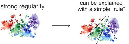 If regularity in the data is strong,
it can be explained with a "simple rule" (i.e., a small probing model).
A small probing model is easy to communicate, i.e., only a few parameters require high precision.
As we will see in the experiments,
similar probe accuracies often come at a very different model cost, i.e. different total codelength.
Note that the variational code gives us probe architecture (and model size) as a
byproduct of training, and does not require
manual search over probe hyperparameters.
If regularity in the data is strong,
it can be explained with a "simple rule" (i.e., a small probing model).
A small probing model is easy to communicate, i.e., only a few parameters require high precision.
As we will see in the experiments,
similar probe accuracies often come at a very different model cost, i.e. different total codelength.
Note that the variational code gives us probe architecture (and model size) as a
byproduct of training, and does not require
manual search over probe hyperparameters.
Online Code: Implicit Transmission of the Model
Online code provides a way to transmit data without directly transmitting the model. Intuitively, it measures the ability to learn from different amounts of data.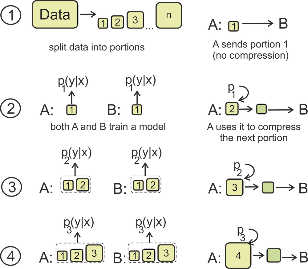 In this setting, the data is transmitted in
a sequence of portions; at each step, the data transmitted so far is used to understand the regularity
in this data and compress the following portion.
In this setting, the data is transmitted in
a sequence of portions; at each step, the data transmitted so far is used to understand the regularity
in this data and compress the following portion.
Codelength: Formal Derivations
Formally, Alice and Bob agree on the form of the model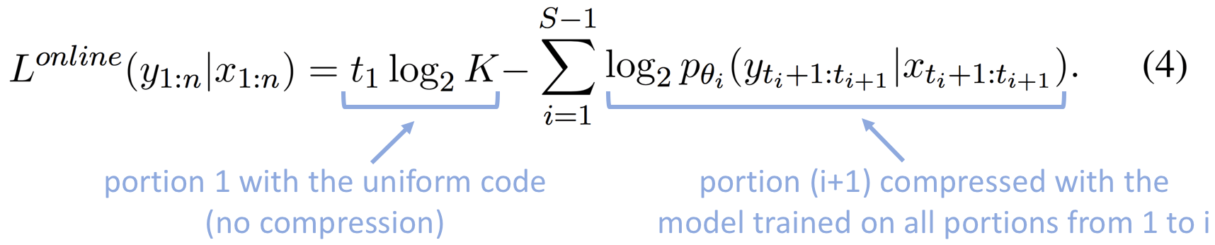
Data and Model components of Online Code
While the online code does not incorporate model cost explicitly, we can still evaluate model cost by interpreting the difference between the cross-entropy of the model trained on all data,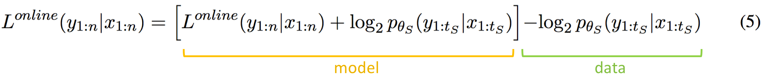
Intuition
 Online code
measures the ability to learn from different amounts of data, and
it is related to the area under the learning curve, which plots quality
as a function of the number of training examples.
Intuitively, if the regularity in the data is strong, it can be
revealed
using a small subset of the data, i.e., early in the transmission process, and can be exploited to efficiently
transmit the rest of the dataset.
Online code
measures the ability to learn from different amounts of data, and
it is related to the area under the learning curve, which plots quality
as a function of the number of training examples.
Intuitively, if the regularity in the data is strong, it can be
revealed
using a small subset of the data, i.e., early in the transmission process, and can be exploited to efficiently
transmit the rest of the dataset.
Description Length and Control Tasks
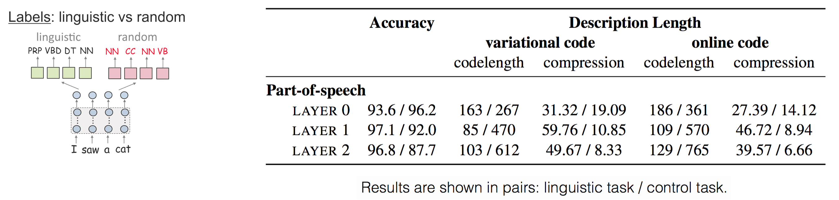
Compression methods agree in results:
- for the linguistic task, the best layer is the first;
- for the control task, codes become larger as we move up from the embedding layer (this is expected since the control task measures the ability to remember word types);
- codelengths for the control task are substantially larger than for the linguistic task.
Layer 0: MDL is correct, accuracy is not.
What is even more surprising, codelength identifies the control task even when accuracy indicates the opposite: for layer 0, accuracy for the control task is higher, but the code is twice longer than for the linguistic task. This is because codelength characterizes how hard it is to achieve this accuracy: for the control task, accuracy is higher, but the cost of achieving this score is very big. We will illustrate this a bit later when looking at the model component of the code.Embedding vs contextual: drastic difference.
For the linguistic task, note that codelength for the embedding layer is approximately twice larger than that for the first layer. Later, when looking at the random model baseline, we will see the same trends for several other tasks and will show that even contextualized representations obtained with a randomly initialized model are a lot better than the embedding layer alone.Model: small for linguistic, large for control.
Let us now look at the data and model components of code separately (as shown in formulas (3) and (5) for variational and online codes, respectively).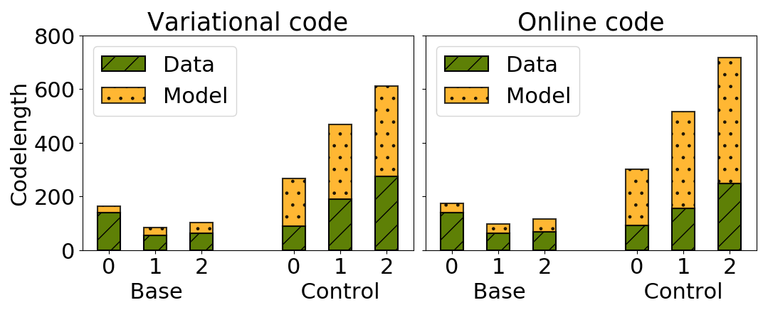 The trends for the two compression methods are similar:
for the control
task, model size is several times larger than for the linguistic task. This is something that
probe accuracy alone is not able to reflect:
while representations have structure with respect to the linguistic task labels,
the same representations do not have structure with
respect to random labels.
For variational code, it means that the linguistic task labels can be "explained"
with a small model, but random labels can be learned only using a larger model.
For online code, it shows that the linguistic task labels can be learned
from a small amount of data, but random labels can be learned (memorized) well only using a large dataset.
The trends for the two compression methods are similar:
for the control
task, model size is several times larger than for the linguistic task. This is something that
probe accuracy alone is not able to reflect:
while representations have structure with respect to the linguistic task labels,
the same representations do not have structure with
respect to random labels.
For variational code, it means that the linguistic task labels can be "explained"
with a small model, but random labels can be learned only using a larger model.
For online code, it shows that the linguistic task labels can be learned
from a small amount of data, but random labels can be learned (memorized) well only using a large dataset.
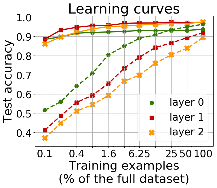 For online code, we can also recall that it is related to the area under the learning curve, which plots quality as a function of the number of training examples.
This figure shows
learning curves corresponding to online code. We can clearly see the difference between behavior of the linguistic and control tasks.
For online code, we can also recall that it is related to the area under the learning curve, which plots quality as a function of the number of training examples.
This figure shows
learning curves corresponding to online code. We can clearly see the difference between behavior of the linguistic and control tasks.
Architecture: sparse for linguistic, dense for control.
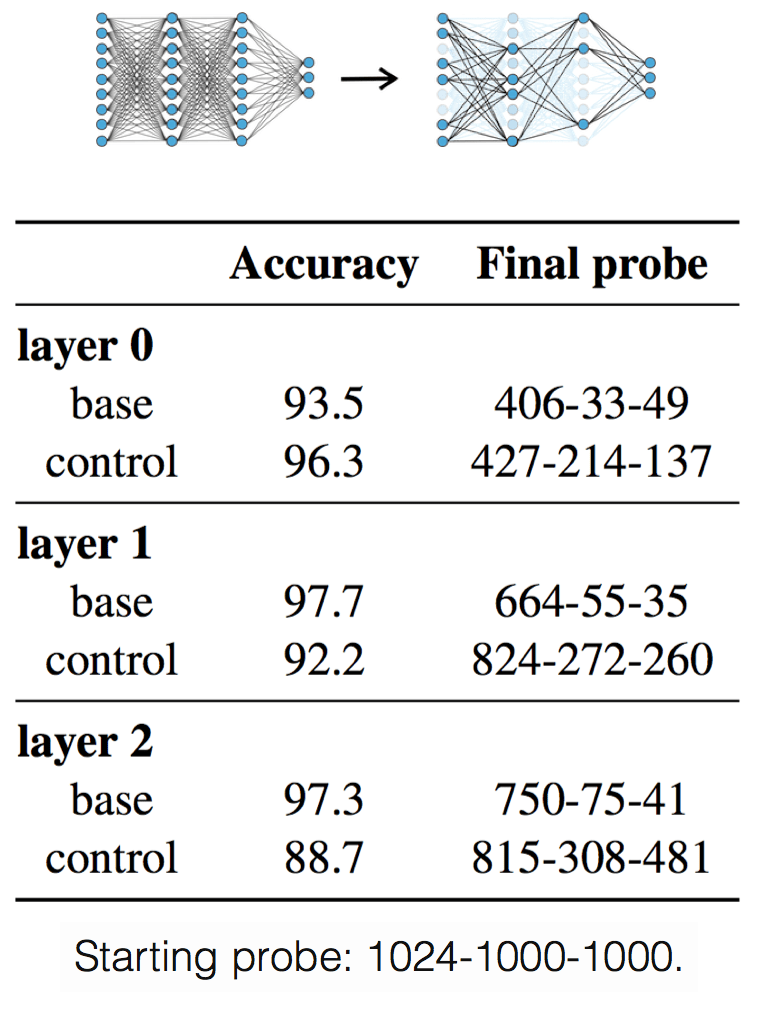 Let us now recall that Bayesian compression
gives us not only variational codelength, but also the induced probe architecture.
Probes learned for linguistic tasks have small architectures with only 33-75 neurons at the second
and third layers of the probe. In contrast, models learned for control tasks are quite dense.
This relates to the control tasks
paper which proposed to use random label baselines.
The authors considered several predefined
probe architectures and picked one of them based on a manually defined criterion. In contrast, variational
code gives probe architecture as a byproduct of training and
does not require human guidance.
Let us now recall that Bayesian compression
gives us not only variational codelength, but also the induced probe architecture.
Probes learned for linguistic tasks have small architectures with only 33-75 neurons at the second
and third layers of the probe. In contrast, models learned for control tasks are quite dense.
This relates to the control tasks
paper which proposed to use random label baselines.
The authors considered several predefined
probe architectures and picked one of them based on a manually defined criterion. In contrast, variational
code gives probe architecture as a byproduct of training and
does not require human guidance.
MDL results are stable, accuracy is not
Hyperparameters: change results for accuracy but not for MDL.
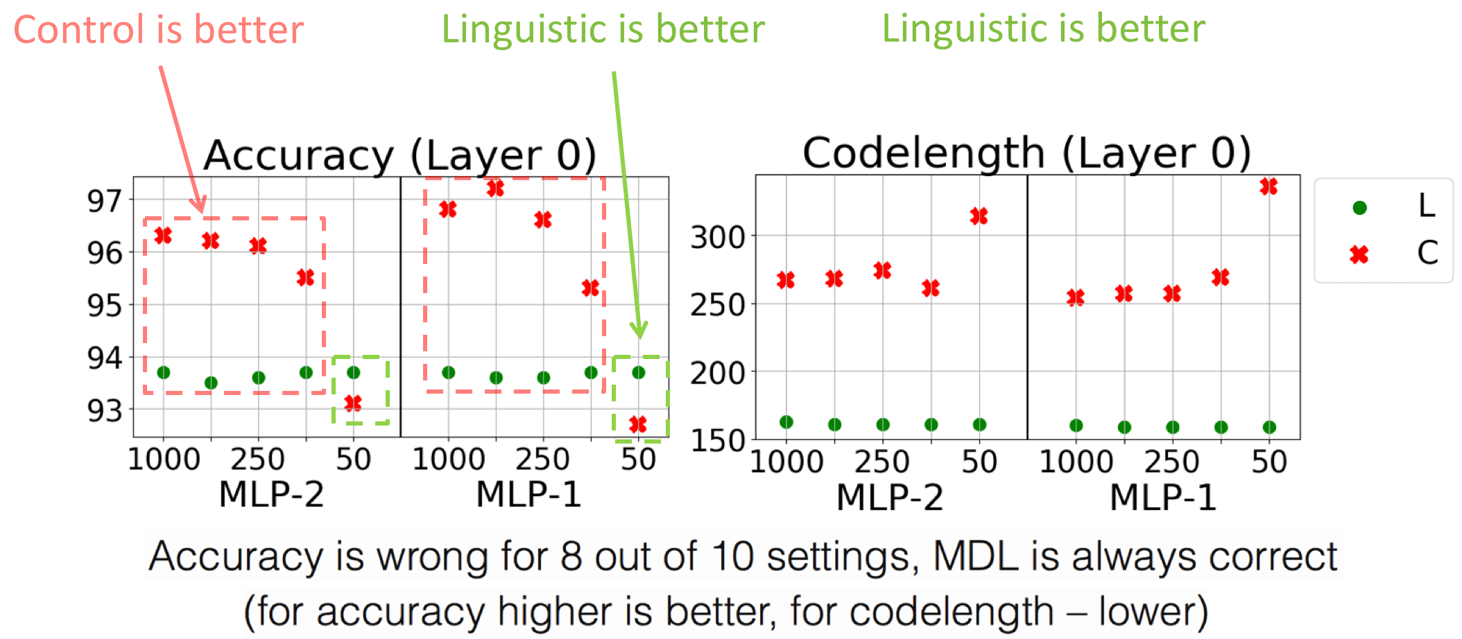 While here we discussed in detail results for the default settings, we also tried
10 different settings and saw that accuracy varies greatly with the settings.
For example, for layer 0 there are settings with contradictory
results: accuracy can be higher either for the linguistic or for the control task depending on the settings
(look at the figure). In striking contrast to accuracy,
MDL results are stable across settings, thus
MDL does not require search for probe settings.
While here we discussed in detail results for the default settings, we also tried
10 different settings and saw that accuracy varies greatly with the settings.
For example, for layer 0 there are settings with contradictory
results: accuracy can be higher either for the linguistic or for the control task depending on the settings
(look at the figure). In striking contrast to accuracy,
MDL results are stable across settings, thus
MDL does not require search for probe settings.
Random Seed: affects accuracy but not MDL.
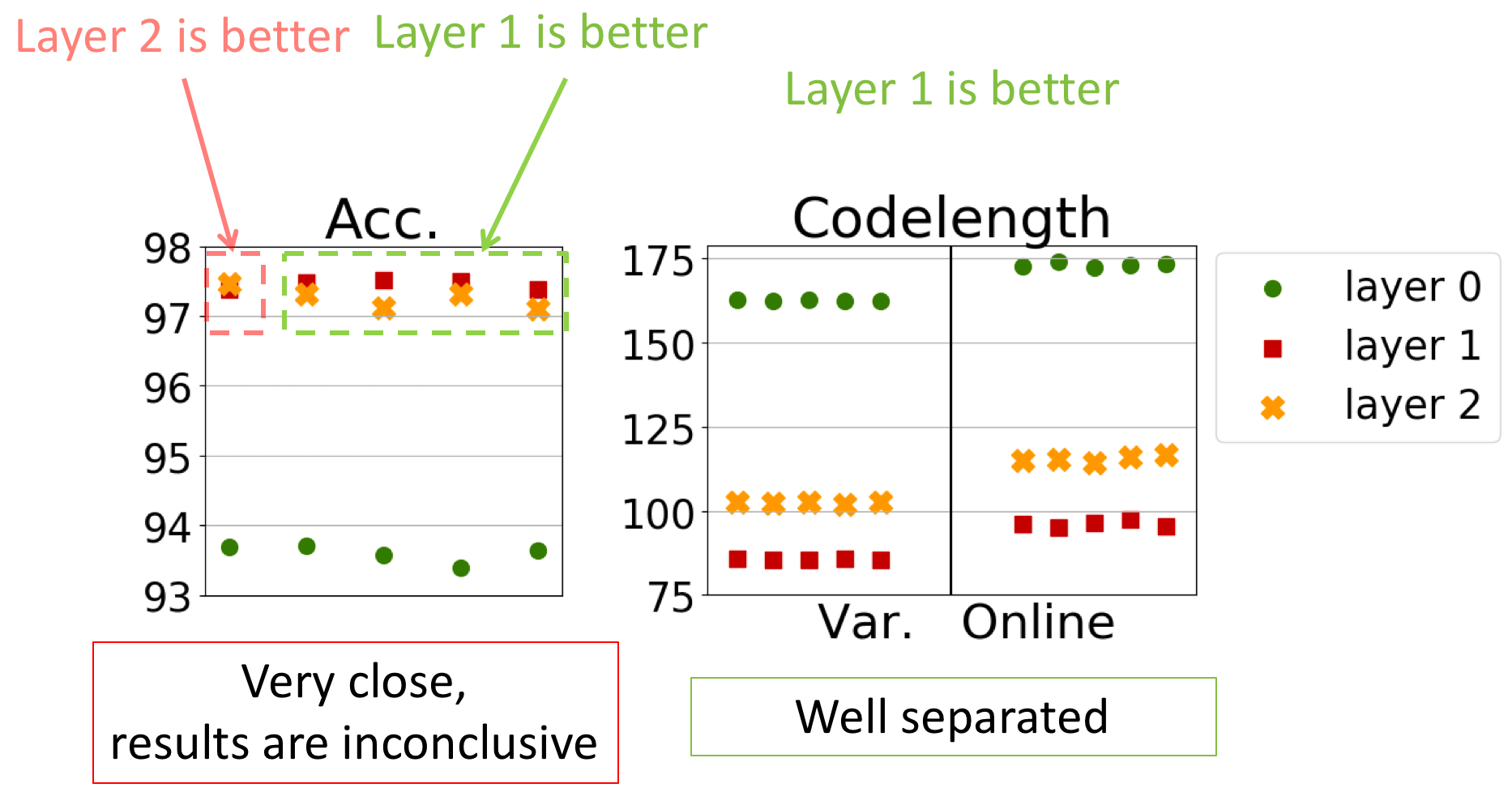 Figure shows results for 5 random seeds (linguistic task).
We see that using accuracy can lead to different
rankings of layers depending on a random seed, making it hard to draw conclusions about their relative qualities.
For example, accuracy for layer 1 and layer 2 are 97.48 and 97.31 for seed 1, but 97.38 and 97.48
for seed 0.
On the contrary, the MDL results are stable and the scores given to different layers are well separated.
Figure shows results for 5 random seeds (linguistic task).
We see that using accuracy can lead to different
rankings of layers depending on a random seed, making it hard to draw conclusions about their relative qualities.
For example, accuracy for layer 1 and layer 2 are 97.48 and 97.31 for seed 1, but 97.38 and 97.48
for seed 0.
On the contrary, the MDL results are stable and the scores given to different layers are well separated.
Description Length and Random Models
 In the paper, we also consider another type of random baselines: randomly initialized models.
Following previous work, we also experiment with ELMo and compare it with a version of the ELMo model in which all weights above the lexical
layer (layer 0) are replaced with random orthonormal matrices (but the embedding layer,
layer 0, is retained from trained ELMo).
We experiment with 7 edge probing tasks (5 of them are listed above).
Here we will only briefly mention our findings: if you are interested in more details, look at the paper.
In the paper, we also consider another type of random baselines: randomly initialized models.
Following previous work, we also experiment with ELMo and compare it with a version of the ELMo model in which all weights above the lexical
layer (layer 0) are replaced with random orthonormal matrices (but the embedding layer,
layer 0, is retained from trained ELMo).
We experiment with 7 edge probing tasks (5 of them are listed above).
Here we will only briefly mention our findings: if you are interested in more details, look at the paper.
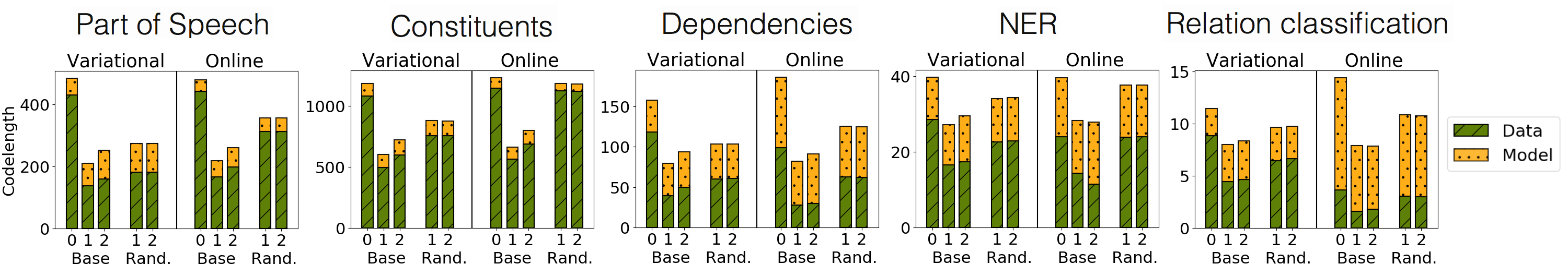
We find, that:
- layer 0 vs contextual: even random contextual representations are better As we already saw in the previous part, codelength shows a drastic difference between the embedding layer (layer 0) and contextualized representations: codelengths differ about twice for most tasks. Both compression methods show that even for the randomly initialized model, contextualized representations are better than lexical representations.
- codelengths for the randomly initialized model are larger than for the trained one This is more prominent when not just looking at the bare scores, but comparing compression against context-agnostic representations. For all tasks, compression bounds for the randomly initialized model are closer to those of context-agnostic Layer 0 than to representations from the trained model. This shows that gain from using context for the randomly initialized model is at least twice smaller than for the trained model.
- randomly initialized layers do not evolve For all tasks, MDL (and data/model components of code separately) for layers of the randomly initialized model is identical. For the trained model, this is not the case: layer 2 is worse than layer 1 for all tasks. This is one more illustration of the general process explained in our Evolution of Representations post: the way representations evolve between layers is defined by the training objective. For the randomly initialized model, since no training objective has been optimized, no evolution happens.
Conclusions
We propose information-theoretic probing which measures minimum description length (MDL) of labels given representations. We show that MDL naturally characterizes not only probe quality, but also the amount of effort needed to achieve it (or, intuitively, strength of the regularity in representations with respect to the labels); this is done in a theoretically justified way without manual search for settings. We explain how to easily measure MDL on top of standard probe-training pipelines. We show that results of MDL probing are more informative and stable compared to the standard probes. Want to know more?
Share: Tweet